机器学习 正则化l1怎么用_机器学习的基础实现（五）：权重衰减（L2正则化）...

这一次主要介绍一个相对常见的应对过拟合的方法：权重衰减。当然，应对过拟合的最好办法是扩大有效样本，这一点尤其要注意。很多时候，没有什么办法比优化自己的样本数据集更加有效，机器学习做多了之后，有时我们常常过于重视调整损失函数，优化方法或者模型结构这些，而忽视了对原始样本的处理。

回到本次的主题：权重衰减。权重衰减等价于L2范数正则化（regularization）。还有L1和L0范数，其中L2范数应对过拟合最好。多说一句，这里的正则化翻译成“规则化”可能更好理解一些。正则化通过为模型损失函数添加惩罚项使学出的模型参数值较小，是应对过拟合的常用手段。至于为什么添加了正则项就能降低过拟合。简单来说，添加了正则项后，损失函数计算梯度下降时就要同时满足原损失函数和正则项的权重同时等于0，压缩了解的空间，即对权重w的可能的取值做了限制。举个例子：比如在人脸识别例中加入：“一定要有眼睛，鼻子”，那么这个条件会使得模型去专注于眼睛和鼻子，而更少的注意力放在人是否戴了眼镜。上面提到的限制就是所谓的“正则项”。具体的数学原理就不在这里详细解释了，本文主要讨论的是代码层面的实现方法。

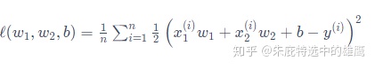
还是以线性回归的函数举例，在没添加正则项之前，损失函数为：

添加惩罚项后：

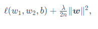
其中超参数λ>0。当权重参数均为0时，惩罚项最小。当λ较大时，惩罚项在损失函数中的比重较大，这通常会使学到的权重参数的元素较接近0。当λ设为0时，惩罚项完全不起作用。上式中L2范数平方∥w∥2展开后得到

下面，我们以高维线性回归为例来引入一个过拟合问题，并使用权重衰减来应对过拟合。设数据样本特征的维度为p。对于训练数据集和测试数据集中特征为x1,x2,…,xp​的任一样本，我们使用如下的线性函数来生成该样本的标签：

其中噪声项ϵ服从均值为0，标准差为0.01的正态分布。为了较容易地观察过拟合，我们考虑高维线性回归问题，如设维度p=200；同时，我们特意把训练数据集的样本数设低，如20。

构造数据：

import tensorflow as tf
# import tensorflow_addons as tfa
from tensorflow.keras import layers, models, initializers, optimizers
import numpy as np
import matplotlib.pyplot as plt

n_train, n_test, num_inputs = 20, 100, 200
true_w, true_b = tf.ones((num_inputs, 1)) * 0.01, 0.05

features = tf.random.normal(shape=(n_train + n_test, num_inputs))
labels = tf.keras.backend.dot(features, true_w) + true_b
labels += tf.random.normal(mean=0.01, shape=labels.shape)
train_features, test_features = features[:n_train, :], features[n_train:, :]
train_labels, test_labels = labels[:n_train], labels[n_train:]

从零开始实现：

def init_params(): #初始化权重和偏置
    w = tf.Variable(tf.random.normal(mean=1, shape=(num_inputs, 1)))
    b = tf.Variable(tf.zeros(shape=(1,)))
    return [w, b]

# 下面定义L2范数惩罚项。这里只惩罚模型的权重参数。
def l2_penalty(w):
    return tf.reduce_sum((w**2)) / 2

定义模型，损失函数，梯度下降算法：

def linreg(X, w, b):
    return tf.matmul(X, w) + b

# 在实现中，我们需要把真实值y变形成预测值y_hat的形状。以下函数返回的结果也将和y_hat的形状相同。
def squared_loss(y_hat, y):
    return (y_hat - tf.reshape(y, y_hat.shape)) ** 2 /2

def sgd(params, lr, batch_size, grads): 
    for i, param in enumerate(params):
        param.assign_sub(lr * grads[i] / batch_size) 

定义一下作图函数，便于观察结果：

# 作图函数
%matplotlib inline
%config InlineBackend.figure_format = 'svg'

def semilogy(x_vals, y_vals, x_label, y_label, x2_vals=None, y2_vals=None, legend=None, figsize=(3.5, 2.5)):
    plt.rcParams['figure.figsize'] = figsize
    plt.xlabel(x_label)
    plt.ylabel(y_label)
    plt.semilogy(x_vals, y_vals)
    if x2_vals and y2_vals:
        plt.semilogy(x2_vals, y2_vals, linestyle=':')
        plt.legend(legend)
    plt.show()

定义拟合模型函数：

batch_size, num_epochs, lr = 1, 100, 0.003
loss = squared_loss
optimizer = tf.keras.optimizers.SGD()
train_iter = tf.data.Dataset.from_tensor_slices(
    (train_features, train_labels)).batch(batch_size).shuffle(batch_size)

def fit_and_plot(lambd): #当lambd设为0时，不使用权重衰减
    w, b = init_params()
    train_ls, test_ls = [], []
    for _ in range(num_epochs):
        for X, y in train_iter:
            with tf.GradientTape(persistent=True) as tape:
                tape.watch(X)
                # 添加了L2范数惩罚项
                l = loss(linreg(X, w, b), y) + lambd * l2_penalty(w)
            grads = tape.gradient(l, [w, b])
            sgd([w, b], lr, batch_size, grads)
        train_ls.append(tf.reduce_mean(loss(linreg(train_features, w, b),
                             train_labels)).numpy())
        test_ls.append(tf.reduce_mean(loss(linreg(test_features, w, b),
                            test_labels)).numpy())
    semilogy(range(1, num_epochs + 1), train_ls, 'epochs', 'loss',
                 range(1, num_epochs + 1), test_ls, ['train', 'test'])
    print('L2 norm of w:', tf.norm(w).numpy())

观察一下有无惩罚项的训练结果：

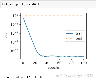
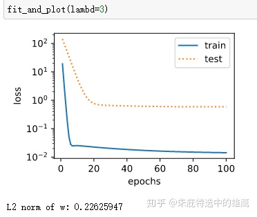
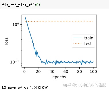
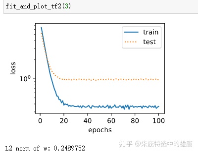
下面是基于tf的简洁实现：

from tensorflow import keras

def fit_and_plot_tf2(wd, lr=1e-3):
    model = models.Sequential()
    model.add(layers.Dense(1, kernel_regularizer=keras.regularizers.l2(wd))) #添加正则化项
    model.build(input_shape=(1, 200))
    w, b = model.trainable_variables
    optimizer = optimizers.SGD(learning_rate=lr)
    
    model.compile(loss='mae', optimizer=optimizer, metrics=['acc'])
    
    history = model.fit(train_features, train_labels,
    batch_size = 1, 
    epochs = 100,
    validation_data = (test_features, test_labels),
    verbose = 0) 
    
    train_ls = history.history['loss']
    test_ls = history.history['val_loss']
    
    semilogy(range(1, num_epochs + 1), train_ls, 'epochs', 'loss',
                 range(1, num_epochs + 1), test_ls, ['train', 'test'])
    print('L2 norm of w:', tf.norm(w).numpy())

结果跟自己实现的差不多：

其实从实际的应用来讲，这部分最主要的还是要理解为什么使用L2正则化能够降低过拟合，实现的过程反而不是那么有意义。我在文章的开头只是定性的大概的讲了一下，并没有很深入，读者有时间应该找资料好好理解一下这部分的内容。