


SphereFace: Deep Hypersphere Embedding for Face Recognition
文章目录
- SphereFace: Deep Hypersphere Embedding for Face Recognition
- Abstract
- 摘要
- 1. Introduction
- 1.介绍
- 2. 相关工作
- 3. Deep Hypersphere Embedding
- 3.深度超球面嵌入
- 4. Experiments (more in Appendix)
- 4.实验(更多见附录)
- 5. Concluding Remarks
- 5. 结束语
-
Appendix(附录)
- A. The intuition of removing the last ReLU
- A.移除最后一个relu层
- B. Normalizing the weights could reduce the prior caused by the training data imbalance
- B.将权重归一化可以减少训练数据不平衡造成的先验问题
- C. Empirical experiment of zeroing out the biases
- C.消除偏差的实验研究
- D. 2D visualization of A-Softmax loss on MNIST
- D. MNIST数据集上A-Softmax loss的二维可视化
- E. Angular Fisher score for evaluating the feature discriminativeness and ablation study on our proposed modifications
- F. Experiments on MegaFace with different convolutional layers
- G. The annealing optimization strategy for A-Softmax loss
- H. Details of the 3-patch ensemble strategy in MegaFace challenge
Abstract
This paper addresses deep face recognition (FR) prob-lem under open-set protocol, where ideal face features are expected to have smaller maximal intra-class distance than minimal inter-class distance under a suitably chosen met-ric space. However, few existing algorithms can effectively achieve this criterion. To this end, we propose the angular softmax (A-Softmax) loss that enables convolutional neural networks (CNNs) to learn angularly discriminative features.Geometrically, A-Softmax loss can be viewed as imposing discriminative constraints on a hypersphere manifold, which intrinsically matches the prior that faces also lie on a mani-fold. Moreover, the size of angular margin can be quantita-tively adjusted by a parameter m. We further derive specificm to approximate the ideal feature criterion. Extensive anal-ysis and experiments on Labeled Face in the Wild (LFW),Youtube Faces (YTF) and MegaFace Challenge show the superiority of A-Softmax loss in FR tasks. The code has also been made publicly available 1 .
摘要
本文讨论了open-set协议下的深度人脸识别问题,在适当选择的度量空间下,理想人脸特征的最大类内距离要小于最小类间距离。然而,现有的算法很少能有效地达到这个标准。为此,我们提出了角度SoftMax(A-SoftMax)损失,它使卷积神经网络(CNN)能够学习角度识别特征。从几何角度来看,A-SoftMax损失可以被视为对超球面流形施加识别约束,超球面流形本质上与前面的面也位于流形上相匹配。此外,可以通过参数m定量调整角度距离的大小。我们进一步推导了近似理想特征准则的具体方法。大量的分析和实验表明了A-SoftMax loss在FR任务中的优势。该代码也已公开发布1。
注:
人脸识别问题,在适当选择的度量空间下,理想人脸特征的最大类内距离要小于最小类间距离。现有的算法很少能有效地达到这个标准。为此提出了角度SoftMax(A-SoftMax)loss,它使卷积神经网络(CNN)能够学习角度识别特征。可以通过参数m定量调整角度间隔的大小。
1. Introduction
Recent years have witnessed the great success of convo-lutional neural networks (CNNs) in face recognition (FR).Owing to advanced network architectures [13, 23, 29, 4] and discriminative learning approaches [25, 22, 34], deep CNNs have boosted the FR performance to an unprecedent level.Typically, face recognition can be categorized as face identi-fication and face verification [8, 11]. The former classifies a face to a specific identity, while the latter determines whether a pair of faces belongs to the same identity.
In terms of testing protocol, face recognition can be eval-uated under closed-set or open-set settings, as illustrated in Fig. 1. For closed-set protocol, all testing identities are predefined in training set. It is natural to classify testing face images to the given identities. In this scenario, face verification is equivalent to performing identification for a pair of faces respectively (see left side of Fig. 1). Therefore, closed-set FR can be well addressed as a classification problem,where features are expected to be separable. For open-set protocol, the testing identities are usually disjoint from the training set, which makes FR more challenging yet close to practice. Since it is impossible to classify faces to known identities in training set, we need to map faces to a discrimi-native feature space. In this scenario, face identification can be viewed as performing face verification between the probe face and every identity in the gallery (see right side of Fig. 1). Open-set FR is essentially a metric learning problem, where the key is to learn discriminative large-margin features.

Closed-set Face Recognition\\\\\\\\\\\\\\\\\\\\\\\ Open-set Face Recognition
Figure 1: Comparison of open-set and closed-set face recognition.
1.介绍
近年来,卷积神经网络在人脸识别中取得了巨大的成功。由于先进的网络体系结构[13、23、29、4]和显著地学习方法[25、22、34],深度CNN将FR性能提升到了前所未有的水平。通常,人脸识别可分为人脸识别和人脸验证[8,11]。前者将一个人脸分类为一个特定的标识,而后者确定一对图片是否属于同一人。
在测试协议方面,人脸识别可以在closed-set 或者open-set 设置下进行评估,如图1所示。对于closed-set协议,所有测试标识都在训练集中预先定义。很自然地将测试人脸图像分类为给定的身份。在这种情况下,人脸验证相当于分别对一对人脸图像进行识别(参见图1左侧)。因此,特征可分时,closed-set FR可以很好地作为一个分类问题来处理。对于open-set协议,测试集通常与训练集分离,这使得FR更具挑战性,但更接近实践。因为不可能将所有人脸图像归纳在一个训练集中,我们需要将人脸映射到一个可辨别的本地特征空间。在这种情况下,人脸识别被视为在输入人脸图片和数据库中的每个身份之间执行人脸验证(参见图1的右侧)。open-set FR本质上是一个度量学习问题,关键是学习具有识别性的大间隔特征。
图1:开集和闭集的人脸识别比较
注:
特征可分时,closed-set FR可以很好地作为一个分类问题来处理。对于open-set协议,测试集通常与训练集分离,这使得FR更具挑战性,但更接近实践。因为不可能将所有人脸图像归纳在一个训练集中,我们需要将人脸映射到一个可辨别的本地特征空间。在这种情况下,人脸识别被视为在输入人脸图像和数据库中的每个身份之间执行人脸验证(参见图1的右侧)。open-set FR本质上是一个度量学习问题,关键是学习具有识别性的大间隔特征。【仔细理解二者的不同,这块的理论分析看图1理解更直观】
Desired features for open-set FR are expected to satisfy the criterion that the maximal intra-class distance is smaller than the minimal inter-class distance under a certain metric space. This criterion is necessary if we want to achieve perfect accuracy using nearest neighbor. However, learning features with this criterion is generally difficult because of the intrinsically large intra-class variation and high inter-class similarity [21] that faces exhibit.
open-set FR期望特征满足一定度量空间下最大类内距离小于最小类间距离的准则。如果我们想使用最近邻实现完美的精度,这个标准是必要的。但是,使用此标准学习特性通常很困难,因为人脸表示出的本质上的较大的类内变化和较高的类间相似性[21]。
Few CNN-based approaches are able to effectively for-mulate the aforementioned criterion in loss functions. Pi-oneering work [30, 26] learn face features via the softmax loss 2 , but softmax loss only learns separable features that are not discriminative enough. To address this, some methods combine softmax loss with contrastive loss [25, 28] or center loss [34] to enhance the discrimination power of features.[22] adopts triplet loss to supervise the embedding learning,leading to state-of-the-art face recognition results. However,center loss only explicitly encourages intra-class compactness. Both contrastive loss [3] and triplet loss [22] can not constrain on each individual sample, and thus require care-fully designed pair/triplet mining procedure, which is both time-consuming and performance-sensitive.
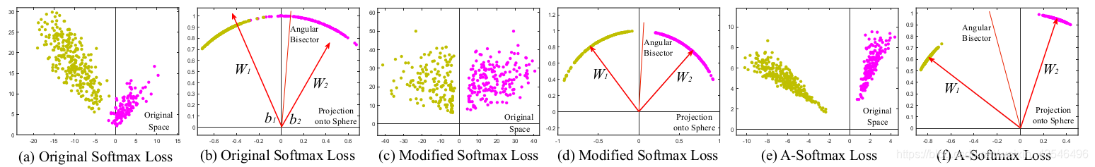 Figure 2: Comparison among softmax loss, modified softmax loss and A-Softmax loss. In this toy experiment, we construct a CNN to learn 2-D features on a subset of the CASIA face dataset. In specific, we set the output dimension of FC1 layer as 2 and visualize the learned features. Yellow dots represent the first class face features, while purple dots represent the second class face features. One can see that features learned by the original softmax loss can not be classified simply via angles, while modified softmax loss can. Our A-Softmax loss can further increase the angular margin of learned features.
很少有基于CNN的方法能够有效地在损失函数中制定上述标准。开创性的工作[30,26]通过SoftMax Loss 2学习面部特征,但SoftMax Loss学习的特征虽然具有可分离性但不具有明显的可判别性。为了解决这一问题,一些方法将SoftMax损失与contrastive loss[25,28]或center loss [34]结合起来,以增强特征的判别能力,[22]采用三重损失来监督嵌入学习,从而获得最先进的人脸识别结果。然而,中心损失只显式地鼓励类内紧凑性。对比损失[3]和三重损失[22]都不能限制在单个样本上,因此需要精心设计的双/三重挖掘过程,这既耗时又对性能敏感。
 图2:Softmax loss、Modified SoftMax loss和A-SoftMax loss之间的比较。在这个验证性的实验中,我们构建了一个CNN来学习CASIA人脸数据集的子集。具体来说,我们将fc1层的输出维度设置为2,并可视化所学的特性。黄色圆点代表第一类人脸特征,而紫色点代表第二类人脸特征。可以看出,原来的SoftMax Loss所学习的特征不能简单地通过角度分类,而修Modified SoftMax loss可以。我们的A-SoftMax loss 可以进一步增加所学特征的角度间隔。
注:
总结softmax loss、contrastive loss、center loss的不足之处,利用实验验证几种loss的角度可分效果。可以从图2明显看出,原始的softmax loss不能简单的通过角度分类,而Modified Softmax loss 明显加强了角度可分性,但不具有高内聚、低耦合的特点,A-Softmax loss则可以达到高内聚、低耦合的特点,而且效果很明显。
It seems to be a widely recognized choice to impose Eu-clidean margin to learned features, but a question arises: Is Euclidean margin always suitable for learning discriminative face features? To answer this question, we first look into how Euclidean margin based losses are applied to FR.
Most recent approaches [25, 28, 34] combine Euclidean margin based losses with softmax loss to construct a joint supervision. However, as can be observed from Fig. 2, the features learned by softmax loss have intrinsic angular dis-tribution (also verified by [34]). In some sense, Euclidean margin based losses are incompatible with softmax loss, so it is not well motivated to combine these two type of losses.
学习特征时增大欧几里得距离,似乎是广泛认可的选择,但问题出现了:欧几里得距离是否总是适合于学习具有可辨别性的面部特征?为了回答这个问题,我们首先研究了基于欧几里得距离的损失如何应用于FR。
最近的方法[25,28,34]将基于欧几里得距离的损失与Softmax loss结合起来,构建一个联合损失函数。然而,如图2所示,由Softmax loss所获得的特征具有固有的角分布(也由[34]验证)。从某种意义上说,基于欧几里得距离的损失与Softmax loss是不相容的,因此将这两种损失结合起来并没有很好的动机。
In this paper, we propose to incorporate angular margin instead. We start with a binary-class case to analyze the softmax loss. The decision boundary in softmax loss is (W 1 − W 2 )x + b 1 − b 2 = 0, where W i and b i are weights and bias 3 in softmax loss, respectively. If we define x as a feature vector and constrain kW 1 k = kW 2 k = 1 and b 1 = b 2 = 0, the decision boundary becomes kxk(cos(θ 1 ) −cos(θ 2 )) = 0, where θ i is the angle between W i and x. The new decision boundary only depends on θ 1 and θ 2 . Modified softmax loss is able to directly optimize angles, enabling CNNs to learn angularly distributed features (Fig. 2).
Compared to original softmax loss, the features learned by modified softmax loss are angularly distributed, but not necessarily more discriminative. To the end, we generalize the modified softmax loss to angular softmax (A-Softmax)loss. Specifically, we introduce an integer m (m ≥ 1) to quantitatively control the decision boundary. In binary-class case, the decision boundaries for class 1 and class 2 become kxk(cos(mθ 1 )−cos(θ 2 ))=0 and kxk(cos(θ 1 )−cos(mθ 2 ))=0, respectively. m quantitatively controls the size of angular margin. Furthermore, A-Softmax loss can be easily generalized to multiple classes, similar to softmax loss.By optimizing A-Softmax loss, the decision regions become more separated, simultaneously enlarging the inter-class margin and compressing the intra-class angular distribution.
在本文中,我们建议用角度距离代替。我们从一个二分类案例开始分析SoftMax loss。SoftMax loss 的决策边界是 ( W 1 − W 2 ) x + b 1 − b 2 = 0 (W_1−W_2)x+b _1−b _2=0 (W1−W2)x+b1−b2=0,其中 W i W_i Wi和 b i b_i bi分别是Softmax loss中的权重和偏差。如果我们将 x x x定义为特征向量并约束 ∣ ∣ W 1 ∣ ∣ = ∣ ∣ W 2 ∣ ∣ = 1 ||W_1||=||W_2|| =1 ∣∣W1∣∣=∣∣W2∣∣=1和 b 1 = b 2 = 0 b_1=b_2=0 b1=b2=0,决策边界变为 ∣ ∣ x ∣ ∣ ( c o s ( θ 1 ) − c o s ( θ 2 ) ) = 0 ||x||(cos(θ_1)−cos(θ_2))=0 ∣∣x∣∣(cos(θ1)−cos(θ2))=0,其中 θ i θ_i θi是 W i W_i Wi和 x x x之间的角度。新的决策边界仅取决于 θ 1 θ_1 θ1和 θ 2 θ_2 θ2。 Modified softmax loss能够直接优化角度,使CNN能够学习角度分布特征(图2)。
与原来的SoftMax loss相比,Modified softmax loss 所学习到的特征是成角度分布的,但不一定更具辨别力。最后,我们归纳出Modified softmax loss到角度SoftMax(A-SoftMax)loss。具体来说,我们引入一个整数m(m≥1)来定量控制决策边界。在二分类的情况下,类1和类2的决策边界分别变为 ∣ ∣ x ∣ ∣ ( c o s ( m θ 1 ) − c o s ( θ 2 ) ) = 0 ||x||(cos(mθ_1)−cos(θ_2))=0 ∣∣x∣∣(cos(mθ1)−cos(θ2))=0和 ∣ ∣ x ∣ ∣ ( c o s ( θ 1 ) − c o s ( m θ 2 ) ) = 0 ||x||(cos(θ_1)−cos(mθ_2))=0 ∣∣x∣∣(cos(θ1)−cos(mθ2))=0。M定量控制角度距离的大小。此外,A-SoftMax loss可以易于推广到多个类,类似于SoftMax loss,通过优化A-SoftMax loss,决策区域变得更加分离,同时扩大了类间损失并压缩了类内角分布。
A-Softmax loss has clear geometric interpretation. Supervised by A-Softmax loss, the learned features construct a discriminative angular distance metric that is equivalent to geodesic distance on a hypersphere manifold. A-Softmax loss can be interpreted as constraining learned features to be discriminative on a hypersphere manifold, which intrin-sically matches the prior that face images lie on a manifold[14, 5, 31]. The close connection between A-Softmax loss and hypersphere manifolds makes the learned features more effective for face recognition. For this reason, we term the learned features as SphereFace.
A-SoftMax loss具有清晰的几何解释。在A-SoftMax loss的监督下,学习特征构造了一个与超球面流形上测地距离相等的角距离判别度量。A-SoftMax loss损失可以解释为限制学习特征在超球面流形上具有识别性,该流形本质上与人脸图像位于流形上之前的图像相匹配[14,5,31]。A-SoftMax loss 和超球面流形之间的紧密联系使得所学特征对于人脸识别更有效。因此,我们将学习到的特征称为球体。
注:
这块翻译的不是很准确,大意应该是将A-SoftMax loss学习到的特征与球体空间的特征进行类比。
Moreover, A-Softmax loss can quantitatively adjust the angular margin via a parameter m, enabling us to do quanti-tative analysis. In the light of this, we derive lower bounds for the parameter m to approximate the desired open-set FR criterion that the maximal intra-class distance should be smaller than the minimal inter-class distance.
Our major contributions can be summarized as follows:
(1) We propose A-Softmax loss for CNNs to learn dis-criminative face features with clear and novel geometric interpretation. The learned features discriminatively spanon a hypersphere manifold, which intrinsically matches the prior that faces also lie on a manifold.
(2) We derive lower bounds for m such that A-Softmax loss can approximate the learning task that minimal inter-class distance is larger than maximal intra-class distance.
(3) We are the very first to show the effectiveness of angular margin in FR. Trained on publicly available CASIA dataset [37], SphereFace achieves competitive results on several benchmarks, including Labeled Face in the Wild (LFW), Youtube Faces (YTF) and MegaFace Challenge 1.
此外,A-SoftMax损耗可以通过参数m定量调整角度间隔,使我们能够进行定量分析。基于此,我们推导出参数m的下界,以近似期望open-set FR标准,即最大类内距离应小于最小类间距离。
我们的主要贡献总结如下:
(1)我们提出A-Softmax loss帮助CNNs去学习具有清晰、新颖的几何解释,可区分性的脸部特征。习得的特征有区别的跨度在一个超球面流形上,它本质上与前面的相匹配,人脸特征也位于流形上。
(2)我们得到了m的下界,这样A-Softmax loss可以完成最小类间距离大于最大类内距离的学习任务。
(3)我们是第一个在FR中证明角度距离的有效性的人。在公开可用的CASIA数据集上进行训练[37],SphereFace在几个基准上得到了具有竞争行为的结果,包括具有标签的Face in the Wild(LFW)、YouTube Faces(YTF)和MegaFace Challenge 1。
注:
但问题出现了:欧几里得距离是否总是适合于学习具有可辨别性的面部特征?从这个问题出发论述了loss 的进阶之路从基于欧几里得的loss与原始Softmax loss结合到(因二者在不同的度量空间)故进阶到Modified softmax loss(因其不具有类间低耦合,类内高内聚的特点)进一步提出A-Softmax loss。
2. 相关工作
度量学习 度量学习旨在学习一个相似的(距离)函数。传统的度量学习[36,38,33,12 ] 常常会学习一个距离度量矩阵A ,在给定的特征
x
1
x_1
x1,
x
2
x_2
x2上距离度量为:
∣
∣
x
1
−
x
2
∣
∣
A
=
[
(
x
1
−
x
2
)
T
A
(
x
1
−
x
2
)
]
1
/
2
||x_1-x_2||_A=[(x_1-x_2)^TA(x_1-x_2)]^{1/2}
∣∣x1−x2∣∣A=[(x1−x2)TA(x1−x2)]1/2
最近流行的深度度量学习[7,17,24,30,25,22,34]通常使用神经网络自动学习具有可区分性的特征
x
1
x_1
x1,
x
2
x_2
x2,然后是简单的进行距离度量,如欧几里得距离
∣
∣
x
1
−
x
2
∣
∣
2
|| x_1−x _2||_2
∣∣x1−x2∣∣2。用于深度度量学习的最广泛的损失函数是对比损失[1,3]和三元组损失[32,22,6],两者都对特征施加欧几里得距离。
Deep face recognition Deep face recognition is arguably one of the most active research area in the past few years. [30, 26] address the open-set FR using CNNs supervised by softmax loss, which essentially treats open-set FR as a multi-class classification problem. [25] combines contrastive loss and softmax loss to jointly supervise the CNNtraining, greatly boosting the performance. [22] uses triplet loss to learn a unified face embedding. Training on nearly 200 million face images, they achieve current state-of-the-art FR accuracy. Inspired by linear discriminant analysis, [34]proposes center loss for CNNs and also obtains promising performance. In general, current well-performing CNNs[28, 15] for FR are mostly built on either contrastive loss or triplet loss. One could notice that state-of-the-art FR methods usually adopt ideas (e.g. contrastive loss, triplet loss)from metric learning, showing open-set FR could be well addressed by discriminative metric learning.
深度人脸识别 深度人脸识别是近几年来最活跃的研究领域之一。[30,26]使用由SoftMax Loss监督的CNN来处理open-set FR,这实质上将open-set FR视为一个多分类问题。[25]将contrastive loss和Softmax loss 相结合,共同监督网络训练,大大提升了性能。[22]使用triplet loss学习统一的人脸编码。利用近2亿张面部图像进行训练,他们实现了目前最好的FR精度。受线性判别分析的启发[34]提出了具有center loss的CNNs网络,而且也获得了良好的性能。一般来说,目前在FR任务表现良好的 CNNs[28,15]主要建立在contrastive loss或triplet loss的基础上。我们可以注意到,最先进的FR方法通常从度量学习的思想中采取想法(例如contrastive loss、triplet loss),显示open-set FR可以通过具有可区分性的度量学习得到很好的解决方案。
L-Softmax loss [16] also implicitly involves the concept of angles. As a regularization method, it shows great improvement on closed-set classification problems. Differently,A-Softmax loss is developed to learn discriminative face embedding. The explicit connections to hypersphere manifold makes our learned features particularly suitable for open-set FR problem, as verified by our experiments. In addition,the angular margin in A-Softmax loss is explicitly imposed and can be quantitatively controlled (e.g. lower bounds to approximate desired feature criterion), while [16] can only be analyzed qualitatively.
L-Softmax loss[16]也隐含了角度的概念。作为一种正则化方法,它在闭集分类问题上显示了很大的进步。不同的是,A-Softmax loss是为了学习具有区分性人脸编码。与超球面流形的具体联系使我们学习的特征特别适合于open-set FR问题,正如我们的实验验证的那样。此外,A-Softmax loss中的角度距离是明确施加的,可以定量控制(例如,近似期望特征标准的下限),而[16]只能定性分析。
注:
1. 人脸识别最开始表现较好好的是基于欧几里得距离的度量学习。
2. 人脸识别开始使用欧几里得loss与softmax loss结合提高了人脸识别的性能。
3. 人脸识别觉得使用欧几里得loss与softmax loss结合的方式无根可寻。
4. 人脸识别开始利用改进的softmax loss进行具有角度距离的度量学习。
3. Deep Hypersphere Embedding
3.1. Revisiting the Softmax Loss
We revisit the softmax loss by looking into the decision criteria of softmax loss. In binary-class case, the posterior probabilities obtained by softmax loss are:
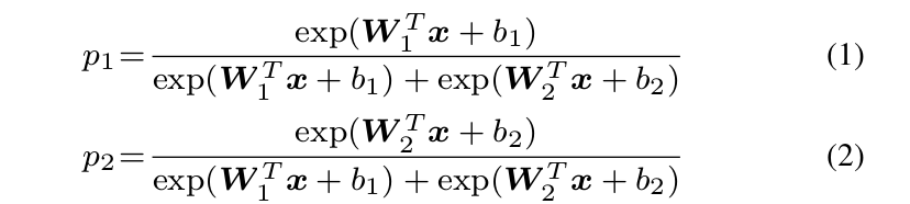
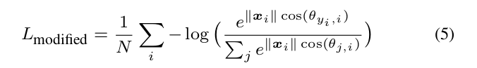
where x is the learned feature vector. W i and b i are weights and bias of last fully connected layer corresponding to class i, respectively. The predicted label will be assigned to class 1 if p 1 > p 2 and class 2 if p 1 < p 2 . By comparing p1 and p2 , it is clear that W 1 T x + b 1 and W 2 T x + b 2 determine the classification result. The decision boundary is(W 1 − W 2 )x + b 1 − b 2 = 0. We then rewrite W i T x + b i as kW i T kkxk cos(θ i ) + b i where θ i is the angle between Wi and x. Notice that if we normalize the weights and zero the biases (kW i k = 1, b i =0), the posterior probabilities become p 1 =kxk cos(θ 1 ) and p 2 =kxk cos(θ 2 ). Note that p 1 and p 2 share the same x, the final result only depends on the angles θ 1 and θ 2 . The decision boundary also becomes cos(θ 1 )−cos(θ 2 )=0 (i.e. angular bisector of vector W 1 and W 2 ). Although the above analysis is built on binary-calss case, it is trivial to generalize the analysis to multi-class case.During training, the modified softmax loss (kW i k=1, b i =0) encourages features from the i-th class to have smaller angle θ i (larger cosine distance) than others, which makes angles between W i and features a reliable metric for classification.
3.深度超球面嵌入
3.1 回顾Softmax Loss
我们通过研究softmax loss的决策标准重新审视softmax loss。在二分类情况下,由softmax loss得到的后验概率为:
其中
x
x
x是学习到的特征向量。
W
i
W_i
Wi和
b
i
b_i
bi分别是对应于i类的最后一个全连接层的权重和偏差。如果
P
1
P_1
P1>
P
2
P_2
P2,预测标签输出为1;如果
P
1
P_1
P1<
P
2
P_2
P2,预测标签输出为2。通过比较
P
1
P_1
P1和
P
2
P_2
P2,很明显
W
1
x
+
b
1
W_1x+b _1
W1x+b1和
W
2
x
+
b
2
W_2x+b_2
W2x+b2决定了分类结果。决策边界是
(
W
1
−
W
2
)
x
+
b
1
−
b
2
=
0
(W_1−W_2)x+b_1−b_2=0
(W1−W2)x+b1−b2=0。然后我们将
W
i
x
+
b
i
W_ix+b_i
Wix+bi重写为
∣
∣
W
i
T
∣
∣
∣
∣
x
∣
∣
c
o
s
(
θ
i
)
+
b
i
||W_i^T||||x||cos(θ_i)+b_i
∣∣WiT∣∣∣∣x∣∣cos(θi)+bi,其中
θ
i
θ_i
θi是
W
i
W_i
Wi和
x
x
x之间的角度。注意,如果我们规范化权重和零偏差(
∣
∣
W
i
∣
∣
=
1
,
b
i
=
0
||W_i||=1,b_i=0
∣∣Wi∣∣=1,bi=0),后验概率为
p
1
=
∣
∣
x
∣
∣
c
o
s
(
θ
1
)
,
p
2
=
∣
∣
x
∣
∣
c
o
s
(
θ
2
)
p_1=||x||cos(θ_1),p_2=||x||cos(θ_2)
p1=∣∣x∣∣cos(θ1),p2=∣∣x∣∣cos(θ2)。注意,
p
1
p_1
p1和
p
2
p_2
p2共享相同的
x
x
x,最终结果只取决于角度
θ
1
θ_1
θ1和
θ
2
θ_2
θ2。决策边界也变成
∣
∣
x
∣
∣
(
c
o
s
(
θ
1
)
−
c
o
s
(
θ
2
)
)
=
0
||x||(cos(θ_1)−cos(θ_2))=0
∣∣x∣∣(cos(θ1)−cos(θ2))=0。尽管上述分析是建立在二元分类上的。也可将分析归纳为多分类任务。在训练过程中,modified softmax loss(
∣
∣
W
i
∣
∣
=
1
,
b
i
=
0
||W_i||=1,b_i=0
∣∣Wi∣∣=1,bi=0)鼓励第i类的特征比其他类具有更小的角度
θ
i
θ_i
θi(更大的余弦距离),这使得
W
i
W_i
Wi和特征之间的角度成为可靠的分类度量。
To give a formal expression for the modified softmax loss,we first define the input feature x i and its label yi . The original softmax loss can be written as:
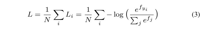
为了给出modified softmax loss表达式,我们首先定义了输入特征
x
i
x_i
xi及其标签
y
i
y_i
yi。原始SoftMax损失可写为:
where f j denotes the j-th element (j ∈ [1, K], K is the class number) of the class score vector f , and N is the number of training samples. In CNNs, f is usually the output of a fully connected layer W , so f j = W j T x i + b j
and f y i = W y T i x i + b y i where x i , W j , W y i are the i-th training sample, the j-th and y i -th column of W respectively.
式中, f j f_j fj表示类得分向量的第j个元素(j∈[1,k],k是类别数),n是训练样本的个数。在CNNs中, f f f通常是完全连接层 W W W的输出,因此 f j = W j T x i + b j f_j=W^T_{j}x_i+b_ j fj=WjTxi+bj和 f y i = W y i T x i + b y i f_{y_i}=W^T_{y_i}x_i+b _{y_i} fyi=WyiTxi+byi,其中 x i x_i xi、 W j W_j Wj、 W y i W_{y_i} Wyi分别是第i个训练样本,参数矩阵W的第集j列和第 y i y_i yi列。
We further reformulate Li in Eq. (3) as
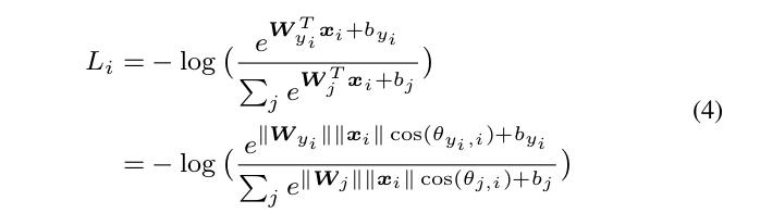
in which θ j,i (0 ≤ θ j,i ≤ π) is the angle between vector W j and x i . As analyzed above, we first normalize kW j k = 1, ∀jin each iteration and zero the biases.
我们进一步将式(3)中的
L
i
L_i
Li重新表述为:
其中
θ
j
,
i
θ_{j,i}
θj,i(
0
≤
θ
j
,
i
≤
π
0≤θ_{j,i}≤π
0≤θj,i≤π)是矢量
W
j
W_j
Wj和
x
i
x _i
xi之间的角度。如前所述,我们首先在每次迭代中归一化
∣
∣
W
j
∣
∣
=
1
||W_j||=1
∣∣Wj∣∣=1,∀j并将偏差归零。
Then we have the modified softmax loss:
Although we can learn features with angular boundary with the modified softmax loss, these features are still not necessarily discriminative. Since we use angles as the distance metric, it is natural to incorporate angular margin to learned features in order to enhance the discrimination power. To this end, we propose a novel way to combine angular margin.
然后我们得到modified softmax loss:
虽然我们可以用具有角度距离的modified softmax loss来学习特征,但这些特征仍然不具有严格的可区分性。因为我们使用角度作为距离度量,所以为了增强辨别力,很自然地将角度间隔应用到特点的学习中。为此,我们提出了一种新的结合角度间隔的方法
注:
利用公式从softmax loss 推导出modified softmax loss,说明我们可以用具有角度间隔的距离度量modified softmax loss来学习特征,但这些特征仍然不具有严格的可区分性,接下来会提出A-Softmax Loss。
3.2. Introducing Angular Margin to Softmax Loss
Instead of designing a new type of loss function and constructing a weighted combination with softmax loss (similar to contrastive loss) , we propose a more natural way to learn angular margin. From the previous analysis of softmax loss, we learn that decision boundaries can greatly affect the feature distribution, so our basic idea is to manipulate decision boundaries to produce angular margin. We first give a motivating binary-class example to explain how our idea works.
3.2. 将角间隔引入Softmax loss
我们提出了一种更自然的方法来学习角度间隔,而不是设计一种新的损失函数或是构造一种与softmax loss(类似于contrastive loss)的加权组合。通过对softmax loss的分析,我们了解到决策边界对特征分布有很大影响。所以我们的基本思想是操纵决策边界产生角度间隔。我们首先给出一个激发性的二元类例子来解释我们的想法是如何工作的。
Assume a learned feature x from class 1 is given and θ i is the angle between x and W i , it is known that the modified softmax loss requires cos(θ 1 ) > cos(θ 2 ) to correctly classify x. But what if we instead require cos(mθ 1 ) > cos(θ 2 ) where m ≥ 2 is a integer in order to correctly classify x? It is essentially making the decision more stringent than previous, because we require a lower bound 4 of cos(θ 1 ) to be larger than cos(θ 2 ). The decision boundary for class 1 is cos(mθ 1 ) = cos(θ 2 ). Similarly, if we require cos(mθ 2 ) >cos(θ 1 ) to correctly classify features from class 2, the decision boundary for class 2 is cos(mθ 2 ) = cos(θ 1 ). Suppose all training samples are correctly classified, such decision1 boundaries will produce an angular margin of m−1m+1 θ 2 where θ21 is the angle between W 1 and W 2 . From angular perspective, correctly classifying x from identity 1 requires θ1 < θ m2 , while correctly classifying x from identity 2 requires θ 2 < θ m 1 . Both are more difficult than original θ 1 < θ 2and θ 2 < θ 1 , respectively. By directly formulating this idea into the modified softmax loss Eq. (5), we have
假设从类别1中得到一个已知的特征
x
x
x,
θ
i
θ_i
θi是
x
x
x和
W
i
W_i
Wi之间的角度,我们知道modified softmax loss需要cos(θ_1)>cos(θ_2)来正确分类
x
x
x。但是如果我们用
c
o
s
(
m
θ
1
)
>
c
o
s
(
θ
2
)
cos(mθ_1)>cos(θ_2)
cos(mθ1)>cos(θ2),其中m≥2是一个整数,是否能正确分类x?它本质上使决策比以前更严格,因为我们要求
c
o
s
(
θ
1
)
cos(θ_1)
cos(θ1)的下界比
c
o
s
(
θ
2
)
cos(θ_2)
cos(θ2)更大。类别1的判定边界是
c
o
s
(
m
θ
1
)
=
c
o
s
(
θ
2
)
cos(mθ_1)=cos(θ_2)
cos(mθ1)=cos(θ2)。同样,如果我们需要
c
o
s
(
m
θ
2
)
>
c
o
s
(
θ
1
)
cos(mθ_2)>cos(θ_1)
cos(mθ2)>cos(θ1)来正确地将从类别2提取的特征分类,那么类别2的决策边界是
c
o
s
(
m
θ
2
)
=
c
o
s
(
θ
1
)
cos(mθ_2)=cos(θ_1)
cos(mθ2)=cos(θ1)。假设所有的训练样本都被正确分类,决策边界将会产生大小为
m
−
1
m
+
1
θ
2
1
{m-1\over m+1}θ_2^1
m+1m−1θ21的角度距离,其中
θ
2
1
θ_2^1
θ21是
W
1
W_1
W1和
W
2
W_2
W2之间的角度。从角度的观点来考虑,从标识1正确分类
x
x
x需要
θ
1
<
θ
2
m
θ_1<{θ_2\over m}
θ1<mθ2,而从标识2正确分类
x
x
x需要
θ
2
<
θ
1
m
θ_2<{θ_1\over m}
θ2<mθ1。两者都比原来的
θ
1
<
θ
2
θ_1<θ_2
θ1<θ2和
θ
2
<
θ
1
θ_2<θ_1
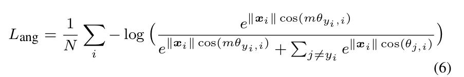
θ2<θ1都困难。在modified softmax loss方程(5)中直接提出这个想法后,我们有
where θ y i ,i has to be in the range of [0, m]. In order to get rid of this restriction and make it optimizable in CNNs,we expand the definition range of cos(θ y i ,i ) by generaliz-ing it to a monotonically decreasing angle function ψ(θ y i ,i )π which should be equal to cos(θ y i ,i ) in [0, m]. Therefore, our proposed A-Softmax loss is formulated as:
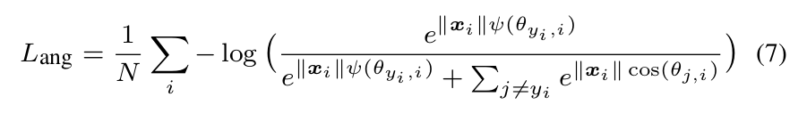
in which we define ψ(θ y i ,i ) = (−1) k cos(mθ y i ,i ) − 2k,(k+1)π θyi ,i ∈ [ kπ] and k ∈ [0, m − 1]. m ≥ 1 is an intem ,m ger that controls the size of angular margin. When m = 1, it becomes the modified softmax loss.
其中 θ y i , i θ_{y_i,i} θyi,i必须在 [ 0 , π m ] [0,{π\over m}] [0,mπ]范围内。为了克服这一限制,使其在CNNs中具有最优性,为了拓展函数的定义域,我们将 c o s ( θ y i , i ) cos(θ_{y_i,i}) cos(θyi,i)推广为单调递减角函数 ψ ( θ y i , i ) ψ(θ_{y_i},i) ψ(θyi,i),在 [ 0 , π m ] [0,{π\over m}] [0,mπ]其值等于 c o s ( θ y i , i ) cos(θ_{y_i,i}) cos(θyi,i)。因此,我们提出的A-SoftMax loss 公式如下:
其中我们定义了
ψ
(
θ
y
i
,
i
)
=
(
−
1
)
k
c
o
s
(
m
θ
y
i
,
i
)
−
2
k
ψ(θ_{y_i,i})=(−1)^k cos(mθ_{y_i},i)−2k
ψ(θyi,i)=(−1)kcos(mθyi,i)−2k,
θ
y
i
,
i
∈
[
k
π
m
,
(
k
+
1
)
π
m
]
θ_{y_i,i}∈[{kπ\over m},{(k+1)π\over m}]
θyi,i∈[mkπ,m(k+1)π],
k
∈
[
0
,
m
−
1
]
k∈[0,m−1]
k∈[0,m−1]。m≥1是一个整数,它控制角度距离的大小。当m=1时,它变为modified softmax loss。
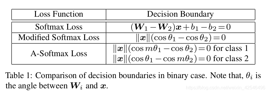
The justification of A-Softmax loss can also be made from decision boundary perspective. A-Softmax loss adopts different decision boundary for different class (each boundary
is more stringent than the original), thus producing angular margin. The comparison of decision boundaries is given in Table 1. From original softmax loss to modified softmax loss, it is from optimizing inner product to optimizing angles. From modified softmax loss to A-Softmax loss, it makes the decision boundary more stringent and separated. The
angular margin increases with larger m and be zero if m = 1.
也可以从决策边界的角度来论证A-Softmax loss的合理性。A-Softmax loss针对不同的类别采用不同的判定边界(每个边界比原始边界更严格),从而产生角度间隔。决策边界的比较见表1。从原始的Softmax loss到modified softmax loss,从优化内积到优化角度。从modified softmax loss到A-Softmax loss,使得决策边界更加严格和分离。角度距离随着m的增大而增大,如果m=1,则为零。
Supervised by A-Softmax loss, CNNs learn face features with geometrically interpretable angular margin. Because A-Softmax loss requires W i = 1, b i = 0, it makes the prediction only depends on angles between the sample x and W i . So x can be classified to the identity with smallest angle. The parameter m is added for the purpose of learning an angular margin between different identities.
To facilitate gradient computation and back propagation, we replace cos(θ j,i ) and cos(mθ y i ,i ) with the expressions only containing W and x i , which is easily done by definition of cosine and multi-angle formula (also the reason why we need m to be an integer). Without θ, we can compute derivative with respect to x and W , similar to softmax loss.
在A-Softmax loss的监督下,CNNs 学习具有几何可解释角度距离的人脸特征。由于A-Softmax loss要求 ∣ ∣ W i ∣ ∣ = 1 ||W_i||=1 ∣∣Wi∣∣=1, b i = 0 b_i=0 bi=0,因此预测只取决于样本 x x x和 W i W_i Wi之间的角度。所以 x x x可以被分类为具有最小角度的特性中。增加参数m目的是为了学习不同特性之间的角度间隔。为了便于梯度计算和反向传播,我们将 c o s ( θ j , i ) cos(θ_{j,i}) cos(θj,i)和 c o s ( m θ j , i ) cos(mθ_{j,i}) cos(mθj,i)替换为仅包含W和 x i x_i xi的表达式,这很容易通过定义cosine和多角度公式(也是我们需要m为整数的原因)来实现。没有θ我们可以计算x和w的导数,类似于softmax loss。
注:
1. modified softmax loss用
c
o
s
(
θ
1
)
>
c
o
s
(
θ
2
)
cos(θ_1)>cos(θ_2)
cos(θ1)>cos(θ2)来正确分类。
2. A-Softmax loss用
c
o
s
(
m
θ
1
)
>
c
o
s
(
θ
2
)
cos(mθ_1)>cos(θ_2)
cos(mθ1)>cos(θ2),m≥2是一个整数。
3. 训练样本都被正确分类时决策边界将会产生大小为
m
−
1
m
+
1
θ
2
1
{m-1\over m+1}θ_2^1
m+1m−1θ21的角度距离,其中
θ
2
1
θ_2^1
θ21是
W
1
W_1
W1和
W
2
W_2
W2之间的角度。
4. 从原始的Softmax loss到modified softmax loss,从优化内积到优化角度。从modified softmax loss到A-Softmax loss,使得决策边界更加严格和分离。
3.3. Hypersphere Interpretation of A-Softmax Loss
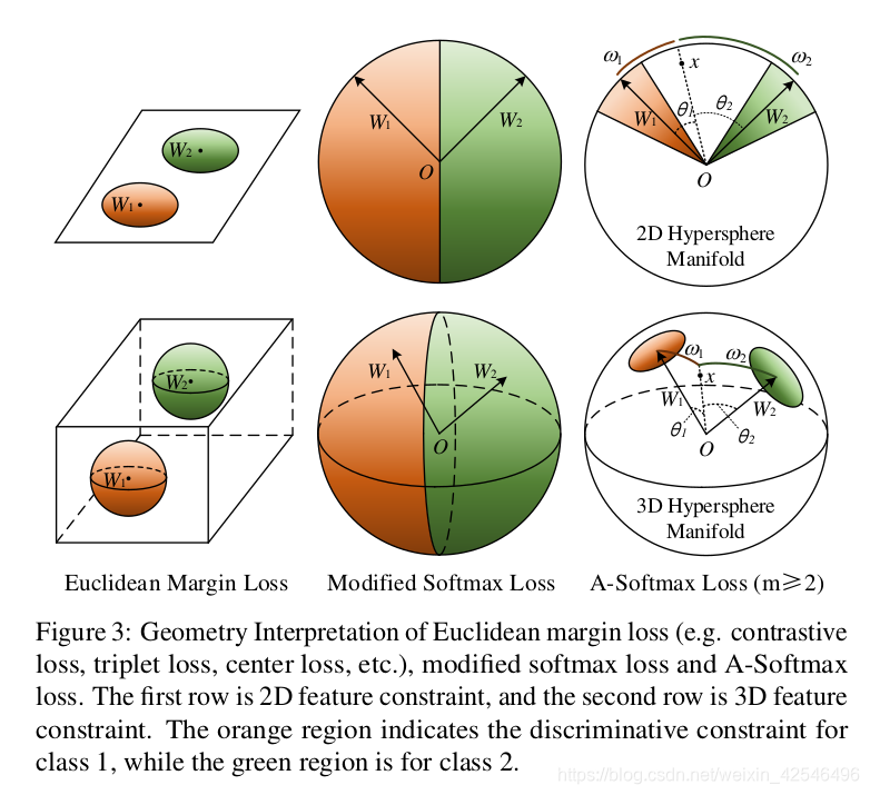
A-Softmax loss has stronger requirements for a correct classification when m ≥ 2, which generates an angular classification margin between learned features of different classes. A-Softmax loss not only imposes discriminative power to the learned features via angular margin, but also renders nice and novel hypersphere interpretation. As shown in Fig. 3,A-Softmax loss is equivalent to learning features that are discriminative on a hypersphere manifold, while Euclidean margin losses learn features in Euclidean space.
3.3 A-Softmax loss的超球面解释
当m≥2时,A-SoftMax损耗对正确分类有更高的要求,不同类别学习到的特征之间产生一个角度分类间隔。A-SoftMax loss不仅通过角间隔对学习到的特征赋予了识别能力,而且还提供了很好的、新颖的超空间解释。如图3所示,a-SoftMax损失相当于在超球面流形上识别的学习特征,而欧几里得边缘损失相当于在欧几里得空间中学习特征。
To simplify, We take the binary case to analyze the hypersphere interpretation. Considering a sample x from class 1 and two column weights W 1 , W 2 , the classification rule forA-Softmax loss is cos(mθ 1 ) > cos(θ 2 ), equivalently mθ 1 <arcθ 2 . Notice that θ 1 , θ 2 are equal to their corresponding P length ω 1 , ω 2 5 on unit hypersphere {v j , ∀j| j v j 2 =1, v≥0}. Because kW k 1 = kW k 2 = 1, the decision replies on the arc length ω 1 and ω 2 . The decision boundary is equivalent to mω 1 = ω 2 , and the constrained region for correctly classifying x to class 1 is mω 1 < ω 2 . Geometrically speaking, this is a hypercircle-like region lying on a hypersphere manifold. For example, it is a circle-like region on the unit sphere in 3D case, as illustrated in Fig. 3. Note that larger m leads to smaller hypercircle-like region for each class, which is an explicit discriminative constraint on a manifold. For better un-derstanding, Fig. 3 provides 2D and 3D visualizations. One can see that A-Softmax loss imposes arc length constraint on a unit circle in 2D case and circle-like region constraint on a unit sphere in 3D case. Our analysis shows that optimizing angles with A-Softmax loss essentially makes the learned features more discriminative on a hypersphere.
注:
这段利用球坐标对A-Softmax loss进行解释,本人不太能理解,所以不具体翻译。
3.4. Properties of A-Softmax Loss
Property 1. A-Softmax loss defines a large angular margin learning task with adjustable difficulty. With larger m,the angular margin becomes larger, the constrained region on the manifold becomes smaller, and the corresponding learning task also becomes more difficult.
We know that the larger m is, the larger angular margin A-Softmax loss constrains. There exists a minimal m that constrains the maximal intra-class angular distance to be smaller than the minimal inter-class angular distance, which can also be observed in our experiments.
3.4. A-Softmax Loss的属性
属性1 A-SoftMax loss定义了一个难度可调的大角度间隔学习任务。随着m的增大,角度间隔变大,流形上的约束区域变小,相应的学习任务也变得更加困难。我们知道,m越大,A-softmax loss约束的角度间隔越大。存在一个最小m,它约束最大类内角度间隔小于最小类间角度间隔,这在我们的实验中也可以观察到。
Definition 1 (minimal m for desired feature distribution).m min is the minimal value such that while m > m min , A-Softmax loss defines a learning task where the maximal intra-class angular feature distance is constrained to be smaller than the minimal inter-class angular feature distance.
定义1(特征分布的最小m)。 m m i n m_{min} mmin是最小值,当 m > m m i n m>m_{min} m>mmin时A-SoftMax loss 定义了一个学习任务,其中最大类内角度特征距离被限制为小于最小类间角度特征距离。
Property 2 (lower bound of m min in binary-class case). In√3binary-class case, we have m min ≥ 2 + 3.Proof. We consider the space spaned by W 1 and W 2 . Because m ≥ 2, it is easy to obtain the maximal angle that classθ 12θ 121 spans is m−1+ m+1where θ 12 is the angle between W 1and W 2 . To require the maximal intra-class feature angular distance smaller than the minimal inter-class feature angular distance, we need to constrain
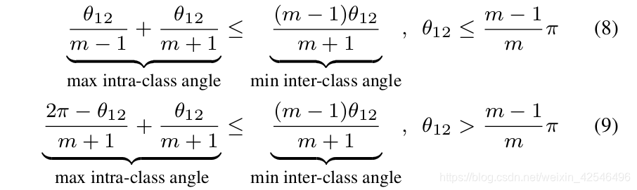 After solving these two inequalities, we could have m min ≥2 +
3
2
\sqrt[2]{3}
23 , which is a lower bound for binary case.
After solving these two inequalities, we could have m min ≥2 +
3
2
\sqrt[2]{3}
23 , which is a lower bound for binary case.
属性2(二分类情况下
m
m
i
n
m_{min}
mmin的下界)。在二分类情况下,
m
m
i
n
m_{min}
mmin ≥2 +
3
2
\sqrt[2]{3}
23。
证明:我们考虑
W
1
W_1
W1和
W
2
W_2
W2的间距。由于m≥2,很容易得到
θ
12
m
−
1
+
θ
12
m
+
1
{θ_{12}\over m-1}+ {θ_{12}\over m+1}
m−1θ12+m+1θ12 ,其中
θ
12
θ_{12}
θ12是
W
1
W_1
W1和
W
2
W_2
W2之间的角度。为了要求最大类内特征角度距离小于最小类间特征角度距离,需要约束
在解决这两个不等式后,我们可以得到
m
m
i
n
m_{min}
mmin≥2+
3
2
\sqrt[2]{3}
23 ,是二分类情况m的下界。
Property 3 (lower bound of m min in multi-class case). Under the assumption that W i , ∀i are uniformly spaced in the Euclidean space, we have m min ≥ 3.
Proof. We consider the 2D k-class (k ≥ 3) scenario for the lower bound. Because W i , ∀i are uniformly spaced in the i+1 2D Euclidean space, we have θ i i+1 = 2π is the k where θ i angle between W i and W i+1 . Since W i , ∀i are symmetric, we only need to analyze one of them. For the i-th class (W i ), We need to constrain
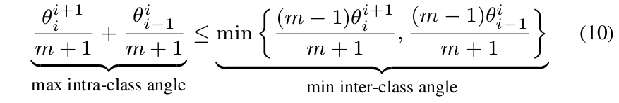
After solving this inequality, we obtain m min ≥ 3, which is a lower bound for multi-class case.
属性3(多类情况下
m
m
i
n
m _{min}
mmin的下界)。假设
W
i
,
∀
i
W_i,∀_i
Wi,∀i在欧几里得空间中均匀分布,我们得到
m
m
i
n
≥
3
m_{min}≥3
mmin≥3。
证明:我们考虑二维空间多分类(k≥3)情形下m的下届。因为
W
i
W_i
Wi,
∀
i
∀_i
∀i在二维欧几里得空间中均匀分布,我们得到
θ
i
i
+
1
=
2
π
k
θ^{i+1}_i={2π\over k}
θii+1=k2π,其中
θ
i
i
+
1
θ^{i+1}_i
θii+1是
W
i
W_i
Wi和
W
i
+
1
W_{i+1}
Wi+1之间的角度。由于
W
i
W_i
Wi,
∀
i
∀_i
∀i是对称的,我们只需要分析其中一个。对于第i类
(
W
i
)
(W_i)
(Wi),我们需要约束:
在解出这个不等式后,得到
m
m
i
n
≥
3
m_{min}≥3
mmin≥3,这是一个多分类情况下m的下界。
Based on this, we use m = 4 to approximate the desired feature distribution criteria. Since the lower bounds are not necessarily tight, giving a tighter lower bound and a upper bound under certain conditions is also possible, which we leave to the future work. Experiments also show that larger m consistently works better and m = 4 will usually suffice.
基于此,我们使用m=4来近似期望的特征分布标准。由于下界不一定是严格的,所以在一定条件下也可以给出更加严格的下界和上界,这将留给以后的工作。实验还表明,较大的m通常工作得更好,m=4通常就足够了。
注:
1. 为了满足最大类内距离小于最小类间距离的要求,对m的值是有要求的(既m的下界)
2. 二分类:
m
m
i
n
≥
2
m_{min}≥2
mmin≥2 +
3
2
\sqrt[2]{3}
23
3. 多分类:
m
m
i
n
≥
3
m_{min}≥3
mmin≥3
3.5. Discussions
Why angular margin. First and most importantly, angular margin directly links to discriminativeness on a manifold,which intrinsically matches the prior that faces also lie on a manifold. Second, incorporating angular margin to softmax loss is actually a more natural choice. As Fig. 2 shows,features learned by the original softmax loss have an intrinsic angular distribution. So directly combining Euclidean margin constraints with softmax loss is not reasonable.
3.5. 讨论
为什么是角角度间隔。首先且最重要的是,角度间隔直接与流形上的区别性联系在一起,流形上的区别性本质上与前面的一致,面也位于流形上。其次,将角度间隔与Softmax loss结合起来实际上是更自然的选择。如图2所示,由原始Softmax loss获得的特征具有固有的角分布。因此,直接将欧几里得间隔约束与Softmax loss 相结合是不合理的。
Comparison with existing losses. In deep FR task, the most popular and well-performing loss functions include contrastive loss, triplet loss and center loss. First, they only impose Euclidean margin to the learned features (w/o normalization), while ours instead directly considers angular margin which is naturally motivated. Second, both contrastive loss and triplet loss suffer from data expansion when constituting the pairs/triplets from the training set, while ours requires no sample mining and imposes discriminative constraints to the entire mini-batches (compared to contrastive and triplet loss that only affect a few representative pairs/triplets).
与已存在的损失进行比较。在深度FR任务中,最流行和性能良好的损失函数包括contrastive loss、 triplet loss 和center loss。首先,它们只将欧几里得距离强加于学习到的特征(w/o标准化),而我们的则直接考虑角度间隔。第二,contrastive loss、 triplet loss 在训练集中构成成对/三重集时都会受到数据扩展的影响,而我们的则不需要样本挖掘,并且对整个小批量都施加了可判别性约束(相比之下,对比损失和三重损失只会影响几个具有代表性的成对/三重集)。
注:
1. 解释了为什么将角度度量学习与softmax loss结合,而不是把欧几里得距离与softmax loss结合。
2. contrastive loss、 triplet loss虽说是比较好的基于欧几里得距离的距离度量loss,但是其性能受到数据挖掘过程的影响。
3. center loss只起到缩小类间距离的作用,不具有增大类间距离的效果。
4. A-Softmax Loss 则是从角度距离度量出发,起到了高内聚,低耦合的显著效果。
4. Experiments (more in Appendix)
4.1. Experimental Settings
Preprocessing. We only use standard preprocessing. The face landmarks in all images are detected by MTCNN [39]. The cropped faces are obtained by similarity transformation. Each pixel ([0, 255]) in RGB images is normalized by subtracting 127.5 and then being divided by 128.
4.实验(更多见附录)
4.1.实验设置
预处理 我们只使用标准的预处理。所有图像中的面部标志由MTCNN检测[39]。通过相似变换得到了被裁剪的面。RGB图像中的每个像素([0,255])通过减去127.5然后除以128进行标准化。
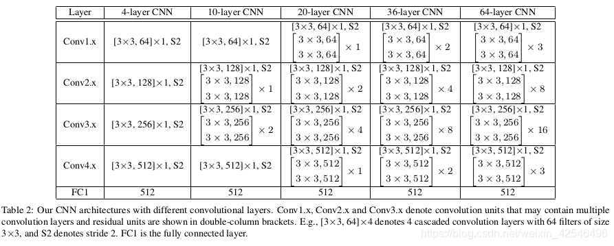
CNNs Setup. Caffe [10] is used to implement A-Softmax loss and CNNs. The general framework to train and extract SphereFace features is shown in Fig. 4. We use residual units [4] in our CNN architecture. For fairness, all compared methods use the same CNN architecture (including residual units) as SphereFace. CNNs with different depths (4, 10, 20, 36, 64) are used to better evaluate our method. The specific settings for difffernt CNNs we used are given in Table 2.According to the analysis in Section 3.4, we usually set m as 4 in A-Softmax loss unless specified. These models are trained with batch size of 128 on four GPUs. The learning rate begins with 0.1 and is divided by 10 at the 16K, 24K iterations. The training is finished at 28K iterations.
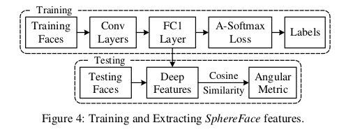
CNN设置 CAffe[10]用于实现A-SoftMax loss 和CNNs。训练和提取SphereFace特征的一般框架如图4所示。我们在CNN架构中使用残差单元[4]。为了公平起见,所有比较的方法都使用相同的CNN架构(包括剩余单元)来来提取sphereFace特征。使用不同深度(4、10、20、36、64)的CNN来更好地评估我们的方法。表2具体的给出了我们使用的不同CNN的设置。根据第3.4节的分析,除非另有规定,否则我们通常在A-SoftMax loss中将m设为4。这些模型在四个GPU上以128的批量大小进行训练。学习率从0.1开始,在16K,24K迭代中除以10。训练以28k次迭代完成。
Training Data. We use publicly available web-collected training dataset CASIA-WebFace [37] (after excluding the images of identities appearing in testing sets) to train our CNN models. CASIA-WebFace has 494,414 face images belonging to 10,575 different individuals. These face images are horizontally flipped for data augmentation. Notice that the scale of our training data (0.49M) is relatively small, especially compared to other private datasets used in DeepFace [30] (4M), VGGFace [20] (2M) and FaceNet [22] (200M).
训练数据 我们使用公共可用训数据集CASIA-WebFace[37](排除测试集中出现的身份图像)来训练我们的CNN模型。CASIA-WebFace共有10575个人的494414张人脸图片。这些人脸图像水平翻转以进行数据增强。请注意,我们的训练数据(0.49m)的规模相对较小,特别是与DeepFace[30](4M)、VggFace[20](2M)和FaceNet[22](200M)中使用的其他私有数据集相比。
Testing. We extract the deep features (SphereFace) from the output of the FC1 layer. For all experiments, the final representation of a testing face is obtained by concatenating its original face features and its horizontally flipped features. The score (metric) is computed by the cosine distance of two features. The nearest neighbor classifier and thresholding are used for face identification and verification, respectively.
测试 我们从fc1层的输出中提取深层特征(SphereFace))。在所有实验中,测试人脸图像的最终表示是通过连接其原始脸部特征和水平翻转特征来获得的。相似度(度量)由两个特征的余弦距离计算。最近邻分类器和阈值分别用于人脸识别和验证。
注:caffe实现
1. 人脸检测部分利用MTCNN实现,预处理中进行了0均值和归一化方差的操作。
2. 利用残差单元搭建网络,A-SoftMax loss中m=4,这些模型在四个GPU上以128的批量大小进行训练。学习率从0.1开始,在16K,24K迭代中除以10。训练以28k次迭代完成。
3. CASIA-WebFace(排除测试集中出现的身份图像)作为训练集来训练我们的CNN模型。
4. 测试时从fc1层的输出中提取深层特征,相似度(度量)由两个特征的余弦距离计算。【注意测试和训练时网络的区别】
4.2. Exploratory Experiments
4.2.探索性实验
4.3. Experiments on LFW and YTF
4.3. 数据集LFW、YTF上的实验
4.4. Experiments on MegaFace Challenge
4.4. MegaFace 挑战上的实验
注:
4.2,4.3,4.4为在一些数据集上对算法效果的验证,这里不具体讨论。
5. Concluding Remarks
This paper presents a novel deep hypersphere embedding approach for face recognition. In specific, we propose the angular softmax loss for CNNs to learn discriminative face features (SphereFace) with angular margin. A-Softmax loss renders nice geometric interpretation by constraining learned features to be discriminative on a hypersphere manifold,which intrinsically matches the prior that faces also lie on a non-linear manifold. This connection makes A-Softmax very effective for learning face representation. Competitive results on several popular face benchmarks demonstrate the superiority and great potentials of our approach. We also believe A-Softmax loss could also benefit some other tasks like object recognition, person re-identification, etc.
5. 结束语
本论文为人脸识别提出了一种新颖的深度超球面嵌入方法。具体地说,我们提出了具有角度特性的softmax loss 来训练CNN进而利用角度间隔来学习具有可辨别性的人脸特征。A-SoftMax loss通过约束学习提供良好的几何解释在超球面流形上具有识别性的特征,它本质上与前面的特征相匹配,面也位于非线性流形上。这种连接使得A-SoftMax对于学习人脸表示非常有效。在多个人脸基准上的竞争结果显示了我们方法的优势和巨大潜力。我们还相信,A-SoftMax loss还可能有助于其他一些任务,如对象识别、人员重新识别等。
Appendix(附录)
A. The intuition of removing the last ReLU
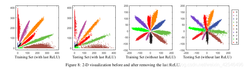
Standard CNNs usually connect ReLU to the bottom of FC1, so the learned features will only distribute in the non-negative range [0, +∞), which limits the feasible learning space (angle) for the CNNs. To address this shortcoming, both SphereFace and [16] first propose to remove the ReLU nonlinearity that is connected to the bottom of FC1 in SphereFace networks. Intuitively, removing the ReLU can greatly benefit the feature learning, since it provides larger feasible learning space (from angular perspective).
Visualization on MNIST. Fig. 8 shows the 2-D visualization of feature distributions in MNIST with and without the last ReLU. One can observe with ReLU the 2-D feature could only distribute in the first quadrant. Without the last ReLU, the learned feature distribution is much more reasonable.
A.移除最后一个relu层
标准CNNs通常将relu连接到fc1的底部,因此所学习的特性将只分布在非负分布中,范围为[0,+∞),这限制了CNN的学习空间(角度)。为了解决这个缺点,SphereFace提出消除SphereFace 网络中连接到fc1底部的relu非线性。直观地说,删除relu可以大大有利于特征学习,因为它提供了更大的可行学习空间(从角度度量学习角度考虑)。
mnist上的可视化 图8显示了mnist中特征分布的二维可视化,分别为包括和不包括最后一个relu操作。在fc1后添加relu激活层,我们可观察到二维特征只能分布在第一象限中。如果没有最后一层的的激活层,学习的特征分布更合理。
B. Normalizing the weights could reduce the prior caused by the training data imbalance
We have emphasized in the main paper that normalizing the weights can give better geometric interpretation. Besides this,we also justify why we want to normalize the weights from a different perspective. We find that normalizing the weights can implicitly reduce the prior brought by the training data imbalance issue (e.g., the long-tail distribution of the training data). In other words, we argue that normalizing the weights can partially address the training data imbalance problem.
B.将权重归一化可以减少训练数据不平衡造成的先验问题
在本文中,我们强调了将权重归一化可以提供更好的几何解释。除此之外,我们还证明了为什么我们要从不同的角度规范化权重。我们发现,将权重归一化可以隐式地减少训练数据不平衡问题(例如训练数据的长尾分布)带来的先验问题。换句话说,我们认为规范化权重可以部分解决训练数据不平衡问题。【属于模型训练的经验问题,一般深度学习课本基本都会介绍】
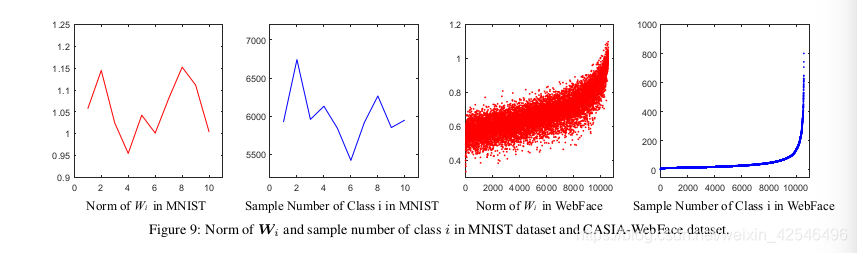
We have an empirical study on the relation between the sample number of each class and the 2-norm of the weights corresponding to the same class (the i-th column of W is associated to the i-th class). By computing the norm of W i and sample number of class i with respect to each class (see Fig. 9), we find that the larger sample number a class has, the larger
the associated norm of weights tends to be. We argue that the norm of weights W i with respect to class i is largely determined by its sample distribution and sample number. Therefore, norm of weights W i , ∀i can be viewed as a learned prior hidden in training datasets. Eliminating such prior is often beneficial to face verification. This is because face verification requires to test on a dataset whose idenities can not appear in training datasets, so the prior from training dataset should not be transferred to the testing. This prior may even be harmful to face verification performance. To eliminate such prior, we normalize the norm of weights of FC2 6 .
我们对每一类的样本数与同一类(W的第i列与第i类相关)权重的2范数之间的关系进行了实证研究。通过计算每个类的
W
i
W_i
Wi范数和i类的样本数(见图9),我们发现一个类的样本数越大,相关的权重范数就越大。我们认为,相对于i类的权重
W
i
W_i
Wi的范数在很大程度上取决于其样本分布和样本数。因此,权重范数
W
i
W_i
Wi,
∀
i
∀_i
∀i可以被视为训练数据集中隐藏的已学先验。消除这种先验通常有利于人脸验证。这是因为人脸验证的测试数据不能在在训练数据集中出现,因此不应将来自训练数据集中的先验问题传输到测试中。这种先验甚至可能对人脸验证性能有害。为了消除这种先验,我们将规范化权重为fc2 。
FC2 refers to the fully connected layer in the softmax loss (or A-Softmax loss).
C. Empirical experiment of zeroing out the biases
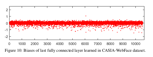
Standard CNNs usually preserve the bias term in the fully connected layers, but these bias terms make it difficult to analyze the proposed A-Softmax loss. This is because SphereFace aims to optimize the angle and produce the angular margin. With bias of FC2, the angular geometry interpretation becomes much more difficult to analyze. To facilitate the analysis, we zero out the bias of FC2 following [16]. By setting the bias of FC2 to zero, the A-Softmax loss has clear geometry interpretation and therefore becomes much easier to analyze. We show all the biases of FC2 from a CASIA-pretrained model in Fig. 10. One can observe that the most of the biases are near zero, indicating these biases are not necessarily useful for face verification.
C.消除偏差的实验研究
标准CNNs通常保留全连接层中的偏置项,但这些偏置项使得分析所提出的A-SoftMax loss 变得困难。这是因为SphereFace的目的是优化角度和产生角度间隔。随着fc2偏置的增大,角度几何解释变得更加困难。为了便于分析,我们在[16]之后将fc2的偏置归零。通过将fc2的偏差设置为零,A-SoftMax loss 具有清晰的几何解释,因此更易于分析。我们在图10中显示了来自CASIA预训练模型的fc2的所有偏差。可以观察到,大多数偏差都接近于零,这表明这些偏差不一定对人脸验证有用
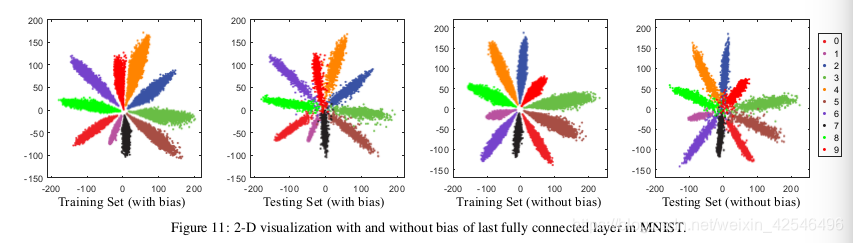
Visualization on MNIST. We visualize the 2-D feature distribution in MNIST dataset with and without bias in Fig. 11.One can observe that zeroing out the bias has no direct influence on the feature distribution. The features learned with and without bias can both make full use of the learning space.
mnist上的可视化 我们将mnist数据集中的二维特征分布在图11中可视化,分别是有偏差和无偏置的。可以观察到,将偏置归零对特征分布没有直接影响。有偏置和无偏置的学习特征都能充分利用学习空间。
D. 2D visualization of A-Softmax loss on MNIST
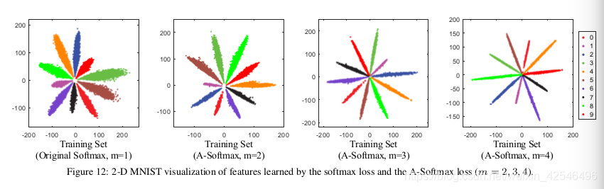
We visualize the 2-D feature distribution on MNIST in Fig. 12. It is obvious that with larger m the learned features become much more discriminative due to the larger inter-class angular margin. Most importantly, the learned discriminative features also generalize really well in the testing set.
D. MNIST数据集上A-Softmax loss的二维可视化
我们将mnist上的二维特征分布可视化,如图12所示。很明显,随着m的增大,学习到的特征由于较大的类间角度间隔而变得更具辨别力。最重要的是,所学到的具有辨别力的特征在测试集中也可以很好地进行归纳
E. Angular Fisher score for evaluating the feature discriminativeness and ablation study on our proposed modifications
F. Experiments on MegaFace with different convolutional layers
G. The annealing optimization strategy for A-Softmax loss
H. Details of the 3-patch ensemble strategy in MegaFace challenge
注:
后面不做具体翻译。


 813
813


 被折叠的 条评论
为什么被折叠?
被折叠的 条评论
为什么被折叠?
 到【灌水乐园】发言


