Survival Analysis with Python 生存分析及Python实现

苏宇-算法交易

已于 2023-11-27 17:16:48 修改

阅读量1.2k

点赞数 1

分类专栏： FinTech # Python 文章标签： python 生存分析生存模型统计学

于 2022-04-03 12:55:09 首次发布

本文链接：https://blog.csdn.net/weixin_42690752/article/details/123907226

版权

Python 同时被 2 个专栏收录

16 篇文章

订阅专栏

FinTech

4 篇文章

订阅专栏

Survival Analysis by Python 生存分析及Python实现

Survival Analysis介绍
- 是什么？可以用来做什么？优势是什么？
- 数学定义
统计检验与模型比较
实验数据
单变量模型 univariate models
生存回归模型
本文的参考链接：

最近学习了Andrew Lo大神的《Econometric Models of Limit-Order Executions》（Journal of Financial Economics，2002），该论文借助Survival Analysis对限价单成交时长进行了建模，借此机会，学习了Survival Analysis的相关内容，记录如下。

总体上看，相比于论文中的分布假设+AFT模型，随着近些年ML的兴起，出现了很多基于ML的Survival Analysis研究。

Survival Analysis介绍

是什么？可以用来做什么？优势是什么？

Survival Analysis是一种统计分析方法，最早由医学研究人员开发使用，用于研究在不同治疗策略下患者的预期寿命，故得此名。

从本质上看，Survival Analysis研究的是在某一特定事件发生前的预期时长（expected duration），所以上面的例子实际上就是研究在death这个事件发生前的预期时长。因此，伴随着对事件的不同定义，Survival Analysis可以用于不同领域。例如，将event定义为客户流失，Survival Analysis可用于对客户留存时长的分析和预测。在Andrew Lo的论文中，event被定义为限价单成交了，于是就可以使用Survival Analysis分析限价单的成交时长。

从以上的内容看，主要目标是预测预期时长，即一个回归问题，那为何要单独提出Survival Analysis这一方法呢？原因是部分数据只能被部分观察到，即出现了censor的现象，例如在研究某种治疗策略的存活时间场景下，某患者在有数据观察的10年里都依然存活或者某患者在10年后退出了研究（观测时长<实际存活时长）。此时，无论是将该患者的存活时间简单截取为10年，还是删去该样本点都是不合适的，都会导致数据被低估。这情况被称为right-censored（实际上还会出现left-censored和interval-censored）。针对包含censor的数据，Survival Analysis中进行了处理，因此特别适用这些场景。在限价单成交时长的场景下，主要是由于有撤单的存在，如果删去这部分撤单的样本，会导致成交时长被低估。

数学定义

Survival Analysis中主要包括S(t)、F(t)、f(t)和h(t)这四个函数。

我们用一个非负、连续随机变量T表示我们的目标，即某一事件发生前的预期时长。例如，客户从订阅到流失的时长、限价单从下单到成交的时长。

T的累积密度函数即CDF用F(t)表示，概率密度函数即PDF用f(t)表示。
事件在t之前发生的概率用F(t)表示，于是有
$\int_0^t f(x)dx$

存活函数用S(t)表示，即事件在t时刻还没有发生的概率，那么显然有
$S(t)=P(T\geq t)=1-F(t)=\int_t^{\infty} f(x)dx \\ S(0)=1 \\ S(x) >= S(y) \quad \forall x\leq y$

除了以上两个函数之外，一般还关心在t时刻事件还没有发生的条件下，事件瞬间发生概率的函数。该函数一般用h(t)表示，被称为hazard function或instantaneous failure rate。从定义上看，首先分母上是一个条件概率（在t时刻事件还没有发生的条件下），分子上强调瞬间发生，是S(t)曲线的斜率，数学上的表示如下所示
$h(t)=\lim_{dt \to 0}\frac{S(t)-S(t+dt)}{dt*S(t)} = \frac{f(t)}{S(t)}$

lifelines文档中的图总结了几个函数之间的关系（还包括了h(t)的CDF）
在这里插入图片描述

从上面的式子中可以看出，S(t)、F(t)、f(t)和h(t)这四个函数之间存在着联系。知道其中一个函数，便能够推出其他函数。下文将借助于这些函数，介绍预测T的相关模型。

统计检验与模型比较

对统计结果进行检验或者比较模型的优劣，有如下方法。

log-rank检验

用于检验两个或多个population的duration之间是否存在统计差异。
在lifelines中的接口有logrank_test()、pairwise_logrank_test()和multivariate_logrank_test()，前两个接口分别用于检验两个或多个population的duration之间是否存在差异，最后一个接口用于检验是否所有的population的duration存在差异。

Survival differences at a point in time

相比于整个曲线上population的差异，有时候我们更关注某个时间点上population的差异，例如医学上不同治疗策略的5年存活期。
在lifelines中的接口有survival_difference_at_fixed_point_in_time_test。

Restricted mean survival times (RMST)

通过比较曲线下的面积，也可以对两个S(t)曲线之间的差异进行评价。注意的是，主要指定t，因为S(t)曲线的尾部往往差异较大。
$RMST(t)=\int_0^tS(r)dr$
在lifelines中的接口有restricted_mean_survival_time。

QQ图

QQ图通过绘制两个概率分布的分位数来进行比较（QQ plot compares the quantiles of our data against the quantiles of the desired distribution），如果比较的两个分布相似，QQ图上的点大约在y=x线上，如果分布是线性相关的，QQ图上的点大约在一条线上，但不一定是在y=x线上。
以判断我们的数据是否符合正态分布为例，首先计算不同分位数和数据的对应值（our quantile），之后计算这些分位数所对应的正态分布中的值（theoretical quantile），之后将theoretical quantile与our quantile一一组合成(x,y)进行画图。显然，如果我们的数据也满足正态分布，(x,y)会落在y=x的直线上。

   percent  our_quantile  theoretical_quantile
0      0.1     -7.011928             -1.281552
1      0.2     -2.963050             -0.841621
2      0.3     -2.659901             -0.524401
3      0.4     -1.975097             -0.253347
4      0.5     -0.848635              0.000000
5      0.6     -0.050281              0.253347
6      0.7      0.124233              0.524401
7      0.8      0.964039              0.841621
8      0.9      2.484332              1.281552

在lifelines中的接口有qq_plot。
QQ图的相关知识可以参与这个链接https://medium.com/towards-data-science/what-in-the-world-are-qq-plots-20d0e41dece1

Log-likelihood

通过在out-of-sample data上的log-likelihood对模型预测效果进行评价。
在lifelines中的接口score返回了the average evaluation of the out-of-sample log-likelihood。

AIC指标 Akaike information criterion

定义一个AIC指标如下，其中k为模型中的参数个数、ll为maximum log-likelihood。因此，模型AIC越低越优。
$A I C (m o d e l) = - 2 ll + 2 k$
在lifelines中的每个模型都有AIC_属性，在Cox中则使用AIC_partial_ 。

Concordance Index 简称为c-index

类似于AUC，用来评价预测时间排序的准确性。数值从0到1，0.5表示随机，一般在0.55到0.75。
在lifelines中，可以在score中指定scoring_method=“concordance_index”，也可以通过模型的concordance_index_属性输出。

实验数据

为了下面的实验，随机生成了如下的一份数据，下列数据读取作为df。
orderIndex表示委托订单编号；
orderBSFlag、orderQty分别表示买卖方向、委托数量；
time-to-first-fill表示从下单到初次成交的时间；（即T）
event_observed表示事件是否被观测到；（1表示观测到了即成交了，0表示未观测到）

OrderIndex	OrderBSFlag	OrderQty	time-to-first-fill	event_observed
1	1	100	1	1
2	2	200	3	1
3	1	200	5	1
4	2	100	7	1
5	1	200	9	1
6	2	100	2	0
7	1	200	4	0
8	2	100	6	0
9	1	200	8	0
10	2	100	10	0

单变量模型 univariate models

使用Kaplan-Meier估计S(t)【非参数方法】

Kaplan-Meier Estimate的数学表达式如下所示，其中 $d_i$ 表示在 $t_i$ 时刻发生的事件数， $n_i$ 表示在 $t_i$ 时刻前处于危险中的受试者数量。
$\hat S(t)= \prod_{t_i\leq t}\frac{n_i-d_i}{n_i}$

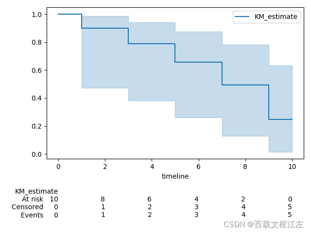
估计S(t)

在实验数据上，S(t)的分布如下所示。

import pandas as pd
from lifelines import KaplanMeierFitter
import matplotlib.pyplot as plt

df = pd.DataFrame([[1, 1, 100, 1, 1],
                   [2, 2, 200, 3, 1],
                   [3, 1, 200, 5, 1],
                   [4, 2, 100, 7, 1],
                   [5, 1, 200, 9, 1],
                   [6, 2, 100, 2, 0],
                   [7, 1, 200, 4, 0],
                   [8, 2, 100, 6, 0],
                   [9, 1, 200, 8, 0],
                   [10, 2, 100, 10, 0]],
                  columns=["OrderIndex", "OrderBSFlag", "OrderQty", "time-to-first-fill", "event_observed"])
kmf = KaplanMeierFitter()
kmf.fit(durations=df["time-to-first-fill"], event_observed=df["event_observed"])
kmf.plot_survival_function(at_risk_counts=True)
print(pd.DataFrame(kmf.survival_function_))
plt.show()

#           KM_estimate
# timeline
# 0.0          1.000000
# 1.0          0.900000
# 2.0          0.900000
# 3.0          0.787500
# 4.0          0.787500
# 5.0          0.656250
# 6.0          0.656250
# 7.0          0.492188
# 8.0          0.492188
# 9.0          0.246094
# 10.0         0.246094

S(1)为0.9的原因是，显然 $d_i$ 为1，根据 $n_i$ 的定义计算的是<1分钟的数量，因此为10，所以为(10-1)/10=0.9。
S(3)为0.7875的原因是，显然 $d_i$ 为1，根据 $n_i$ 的定义计算的是<3分钟的数量，因此为8，所以为0.9*(8-1)/8=0.7875。
在这里插入图片描述
如果使用scikit-survival，则代码如下

import pandas as pd
import matplotlib.pyplot as plt
from sksurv.nonparametric import kaplan_meier_estimator


df = pd.DataFrame([[1, 1, 100, 1, 1],
                   [2, 2, 200, 3, 1],
                   [3, 1, 200, 5, 1],
                   [4, 2, 100, 7, 1],
                   [5, 1, 200, 9, 1],
                   [6, 2, 100, 2, 0],
                   [7, 1, 200, 4, 0],
                   [8, 2, 100, 6, 0],
                   [9, 1, 200, 8, 0],
                   [10, 2, 100, 10, 0]],
                  columns=["OrderIndex", "OrderBSFlag", "OrderQty", "time-to-first-fill", "event_observed"])
df["event_observed"] = df["event_observed"].astype(bool)
time, survival_prob = kaplan_meier_estimator(df["event_observed"], df["time-to-first-fill"])
plt.step(time, survival_prob, where="post")
plt.show()

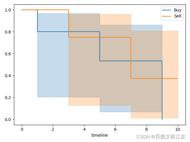
估计不同类别上的S(t)

除此之外，我们还可以引入一个变量，研究S(t)在不同变量上的表现，例如可以研究在买卖不同方向上的time-to-first-fill是否存在差异。

import pandas as pd
from lifelines import KaplanMeierFitter
import matplotlib.pyplot as plt

df = pd.DataFrame([[1, 1, 100, 1, 1],
                   [2, 2, 200, 3, 1],
                   [3, 1, 200, 5, 1],
                   [4, 2, 100, 7, 1],
                   [5, 1, 200, 9, 1],
                   [6, 2, 100, 2, 0],
                   [7, 1, 200, 4, 0],
                   [8, 2, 100, 6, 0],
                   [9, 1, 200, 8, 0],
                   [10, 2, 100, 10, 0]],
                  columns=["OrderIndex", "OrderBSFlag", "OrderQty", "time-to-first-fill", "event_observed"])
kmf = KaplanMeierFitter()
buy_side_index = (df["OrderBSFlag"] == 1)

kmf.fit(durations=df.loc[buy_side_index, "time-to-first-fill"], event_observed=df.loc[buy_side_index, "event_observed"], label="Buy")
kmf.plot_survival_function()

kmf.fit(durations=df.loc[~buy_side_index, "time-to-first-fill"], event_observed=df.loc[~buy_side_index, "event_observed"], label="Sell")
kmf.plot_survival_function()

plt.show()

在这里插入图片描述

log-rank检验

对上面不同买卖方向的time-to-first-fill之间是否存在差异进行检验。

import pandas as pd
from lifelines.statistics import logrank_test

df = pd.DataFrame([[1, 1, 100, 1, 1],
                   [2, 2, 200, 3, 1],
                   [3, 1, 200, 5, 1],
                   [4, 2, 100, 7, 1],
                   [5, 1, 200, 9, 1],
                   [6, 2, 100, 2, 0],
                   [7, 1, 200, 4, 0],
                   [8, 2, 100, 6, 0],
                   [9, 1, 200, 8, 0],
                   [10, 2, 100, 10, 0]],
                  columns=["OrderIndex", "OrderBSFlag", "OrderQty", "time-to-first-fill", "event_observed"])
buy_side_index = (df["OrderBSFlag"] == 1)
results = logrank_test(df.loc[buy_side_index, "time-to-first-fill"],
                       df.loc[~buy_side_index, "time-to-first-fill"],
                       event_observed_A=df.loc[buy_side_index, "event_observed"],
                       event_observed_B=df.loc[~buy_side_index, "event_observed"])
results.print_summary()
print(results.p_value)  # 0.6547208460185768
print(results.test_statistic)   # 0.2

检验结果显示p值为0.65，显然无法拒绝原假设，即实验数据中的买卖方向之间不存在差异，与从图中的观察一致。

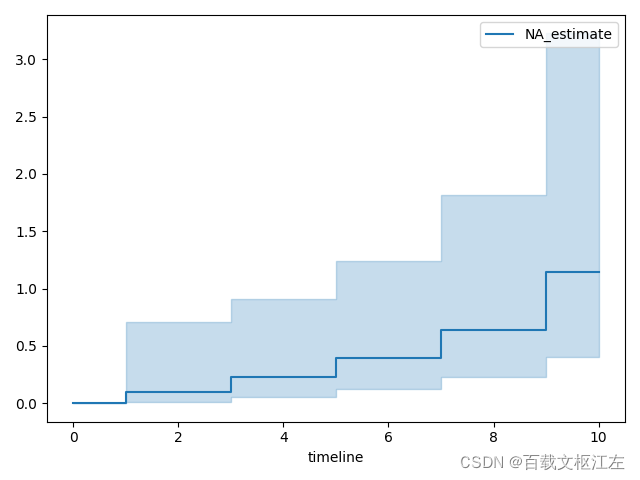
使用Nelson-Aalen估计H(t) 【非参数方法】

除了估计生存函数S(t)之外，我们还可以对hazard function即h(t)，例如使用下面的公式估计h(t)的CDF即H(t)。
$\hat H(t)=\sum_{t_i\leq t}\frac{d_i}{n_i}$
和KM估计中相同， $d_i$ 表示在 $t_i$ 时刻发生的事件数， $n_i$ 表示在 $t_i$ 时刻前处于危险中的受试者数量。

from lifelines import NelsonAalenFitter
import pandas as pd
import matplotlib.pyplot as plt

df = pd.DataFrame([[1, 1, 100, 1, 1],
                   [2, 2, 200, 3, 1],
                   [3, 1, 200, 5, 1],
                   [4, 2, 100, 7, 1],
                   [5, 1, 200, 9, 1],
                   [6, 2, 100, 2, 0],
                   [7, 1, 200, 4, 0],
                   [8, 2, 100, 6, 0],
                   [9, 1, 200, 8, 0],
                   [10, 2, 100, 10, 0]],
                  columns=["OrderIndex", "OrderBSFlag", "OrderQty", "time-to-first-fill", "event_observed"])
naf = NelsonAalenFitter()
naf.fit(df["time-to-first-fill"], event_observed=df["event_observed"])
naf.plot_cumulative_hazard()
plt.show()

在这里插入图片描述

参数方法：Weibull、Exponential,、Log-Logistic、Log-Normal、Splines、Generalized-Gamma模型

相比于K-M和N-A中的非参数方法，我们也可以假定S(t)、H(t)所属的分布，然后用数据求出分布中的参数。
以Weibull为例，需要求解的参数是 $\lambda$ 和 $\rho$
$S(t)=exp(-(\frac{t}{\lambda})^\rho) \\ H(t)=(\frac{t}{\lambda})^{\rho}$

from lifelines import WeibullFitter
import pandas as pd

df = pd.DataFrame([[1, 1, 100, 1, 1],
                   [2, 2, 200, 3, 1],
                   [3, 1, 200, 5, 1],
                   [4, 2, 100, 7, 1],
                   [5, 1, 200, 9, 1],
                   [6, 2, 100, 2, 0],
                   [7, 1, 200, 4, 0],
                   [8, 2, 100, 6, 0],
                   [9, 1, 200, 8, 0],
                   [10, 2, 100, 10, 0]],
                  columns=["OrderIndex", "OrderBSFlag", "OrderQty", "time-to-first-fill", "event_observed"])
wf = WeibullFitter().fit(df["time-to-first-fill"], event_observed=df["event_observed"])
wf.print_summary()
# <lifelines.WeibullFitter:"Weibull_estimate", fitted with 10 total observations, 5 right-censored observations>
#    number of observations = 10
# number of events observed = 5
#            log-likelihood = -16.27
#                hypothesis = lambda_ != 1, rho_ != 1
# 
# ---
#           coef   se(coef)   coef lower 95%   coef upper 95%    z      p   -log2(p)
# lambda_   9.10       2.59             4.03            14.17 3.13 <0.005       9.16
# rho_      1.66       0.63             0.42             2.89 1.04   0.30       1.75
# ---
# AIC = 36.54

使用QQ图、Log-likehood、AIC选择模型

from lifelines import *
from lifelines.plotting import qq_plot
import pandas as pd
import matplotlib.pyplot as plt
import random

ls = [[1, 1, 100, 1, 1],
      [2, 2, 200, 3, 1],
      [3, 1, 200, 5, 1],
      [4, 2, 100, 7, 1],
      [5, 1, 200, 9, 1],
      [6, 2, 100, 2, 0],
      [7, 1, 200, 4, 0],
      [8, 2, 100, 6, 0],
      [9, 1, 200, 8, 0],
      [10, 2, 100, 10, 0]]
ls = [[lss[3] + random.randint(1, 10), lss[4]] for lss in ls for _ in range(100)]
df = pd.DataFrame(ls, columns=["time-to-first-fill", "event_observed"])

fig, axes = plt.subplots(2, 2)
axes = axes.reshape(4, )

for i, model in enumerate([WeibullFitter(), LogNormalFitter(), LogLogisticFitter(), ExponentialFitter()]):
    model.fit(df["time-to-first-fill"], event_observed=df["event_observed"])
    print(model, model.log_likelihood_, model.AIC_)
    qq_plot(model, ax=axes[i])
plt.show()
# <lifelines.WeibullFitter:"Weibull_estimate", fitted with 1000 total observations, 500 right-censored observations> -1816.1656841614129 3636.3313683228257
# <lifelines.LogNormalFitter:"LogNormal_estimate", fitted with 1000 total observations, 500 right-censored observations> -1851.521385280591 3707.042770561182
# <lifelines.LogLogisticFitter:"LogLogistic_estimate", fitted with 1000 total observations, 500 right-censored observations> -1830.8689894251984 3665.7379788503968
# <lifelines.ExponentialFitter:"Exponential_estimate", fitted with 1000 total observations, 500 right-censored observations> -2042.4664595062745 4086.932919012549

在这里插入图片描述

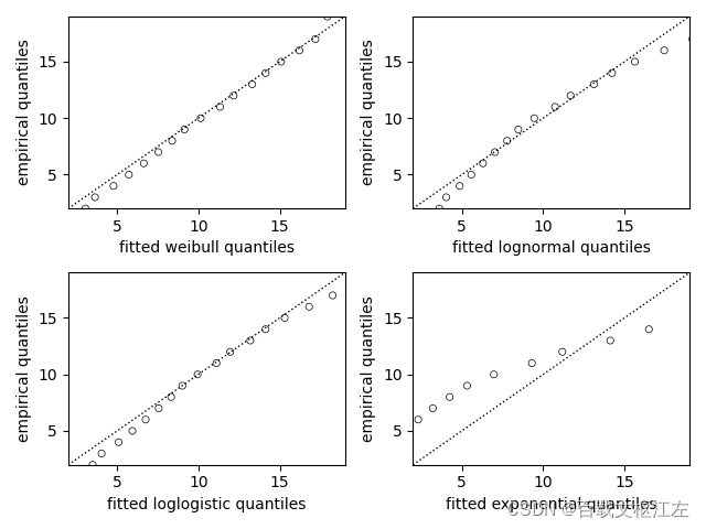
从指标上看，weibull模型更符合随机生成的数据。

生存回归模型

如果想在对S(t)建模时引入一些特征，例如限价单成交时长预测中的下单量特征，就需要使用生存回归模型。类似地，由于censor现象的存在，直接使用回归模型不合适，所以需要使用这里的生存回归模型。

Cox proportional hazard模型

Cox模型假设特征对h(t)有线性倍增效应，并且该效应随时间推移保持不变。
$H(t|x)=exp(x^T\beta)\int_0^t h_0(s)ds$
相比于fully parametric models，Cox Proportional Hazards regression这种semi-parametric models的优点在于不需要知道或假设数据所属的分布

from lifelines import CoxPHFitter
import pandas as pd
import matplotlib.pyplot as plt

df = pd.DataFrame([[1, 1, 100, 1, 1],
                   [2, 2, 200, 3, 1],
                   [3, 1, 200, 5, 1],
                   [4, 2, 100, 7, 1],
                   [5, 1, 200, 9, 1],
                   [6, 2, 100, 2, 0],
                   [7, 1, 200, 4, 0],
                   [8, 2, 100, 6, 0],
                   [9, 1, 200, 8, 0],
                   [10, 2, 100, 10, 0]],
                  columns=["OrderIndex", "OrderBSFlag", "OrderQty", "time-to-first-fill", "event_observed"])
df = df.drop(columns=["OrderIndex"])
cph = CoxPHFitter()
cph.fit(df, duration_col='time-to-first-fill', event_col='event_observed')
cph.print_summary()
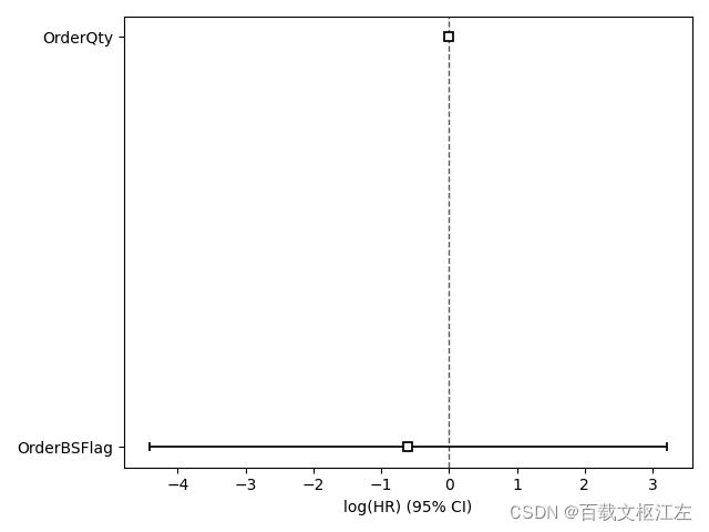
cph.plot()
# 测试单变量对生存曲线的影响
cph.plot_partial_effects_on_outcome(covariates='OrderBSFlag', values=[1, 2], cmap='coolwarm', plot_baseline=False)
plt.show()

# <lifelines.CoxPHFitter: fitted with 10 total observations, 5 right-censored observations>
#              duration col = 'time-to-first-fill'
#                 event col = 'event_observed'
#       baseline estimation = breslow
#    number of observations = 10
# number of events observed = 5
#    partial log-likelihood = -8.15
#
# ---
#               coef  exp(coef)   se(coef)   coef lower 95%   coef upper 95%  exp(coef) lower 95%  exp(coef) upper 95%
# covariate
# OrderBSFlag  -0.60       0.55       1.94            -4.41             3.21                 0.01                24.66
# OrderQty     -0.00       1.00       0.02            -0.04             0.04                 0.96                 1.04
#
#                 z    p   -log2(p)
# covariate
# OrderBSFlag -0.31 0.76       0.40
# OrderQty    -0.12 0.91       0.14
# ---
# Concordance = 0.58
# Partial AIC = 20.29
# log-likelihood ratio test = 0.21 on 2 df
# -log2(p) of ll-ratio test = 0.16

在这里插入图片描述

Accelerated failure time模型 AFT模型

$H(t|x)=(\frac{t}{exp(x^T\beta)})^\rho$
lifelines中有WeibullAFTFitter接口，另外可以指定ancillary参数如为True同时对 $\rho$ 进行建模。
另外还有LogNormalAFTFitter、LogLogisticAFTFitter和 GeneralizedGammaRegressionFitter。

Aalen’s additive model

$h(t|x)=b_0(t)+b_1(t)x_1+...+b_N(t)x_N$
lifelines中有AalenAdditiveFitter接口

模型保存

from lifelines.utils.sklearn_adapter import sklearn_adapter
from lifelines import CoxPHFitter
sklearn_adapter(CoxPHFitter, event_col='arrest')

from joblib import load

model = load(...)


from dill import loads, dumps
from pickle import loads, dumps

s_cph = dumps(cph)
cph_new = loads(s_cph)
cph_new.summary
s_kmf = dumps(kmf)
kmf_new = loads(s_kmf)
kmf_new.survival_function_


import pickle
with open('/path/my.pickle', 'wb') as f:
    pickle.dump(cph, f) # saving my trained cph model as my.pickle
with open('/path/my.pickle', 'rb') as f:
    cph_new = pickle.load(f)
cph_new.summary # should produce the same output as cph.summary

使用scikit-survival做gridsearch

相比于lifelines库，scikit-survival库提供了更多近似于scikit-learn的工具

from sksurv.linear_model import CoxPHSurvivalAnalysis
from sklearn.model_selection import GridSearchCV, KFold
import pandas as pd
pd.set_option("display.max_columns", None)

df = pd.DataFrame([[1, 1, 100, 1, 1],
                   [2, 2, 200, 3, 1],
                   [3, 1, 200, 5, 1],
                   [4, 2, 100, 7, 1],
                   [5, 1, 200, 9, 1],
                   [6, 2, 100, 2, 0],
                   [7, 1, 200, 4, 0],
                   [8, 2, 100, 6, 0],
                   [9, 1, 200, 8, 0],
                   [10, 2, 100, 10, 0]],
                  columns=["OrderIndex", "OrderBSFlag", "OrderQty", "time-to-first-fill", "event_observed"])
df["event_observed"] = df["event_observed"].astype(bool)
df = df.drop(columns=["OrderIndex"])
data_x, data_y = df[["OrderBSFlag", "OrderQty"]], df[["event_observed", "time-to-first-fill"]]
data_y = data_y.to_records(index=False)

param_grid = {'alpha': [1, 100, 1000]}
cv = KFold(n_splits=2, random_state=1, shuffle=True)
gcv = GridSearchCV(CoxPHSurvivalAnalysis(), param_grid, return_train_score=True, cv=cv)
gcv.fit(data_x, data_y)

results = pd.DataFrame(gcv.cv_results_).sort_values(by='mean_test_score', ascending=False)
results = results.loc[:, ~results.columns.str.endswith("_time")]
print(results)
#   param_alpha           params  split0_test_score  split1_test_score  \
# 1         100   {'alpha': 100}           0.071429                0.5
# 2        1000  {'alpha': 1000}           0.071429                0.5
# 0           1     {'alpha': 1}           0.071429                0.0
#
#    mean_test_score  std_test_score  rank_test_score  split0_train_score  \
# 1         0.285714        0.214286                1                 1.0
# 2         0.285714        0.214286                1                 1.0
# 0         0.035714        0.035714                3                 1.0
#
#    split1_train_score  mean_train_score  std_train_score
# 1            0.500000          0.750000         0.250000
# 2            0.500000          0.750000         0.250000
# 0            0.928571          0.964286         0.035714

基于ML的模型

随机森林
sksurv.ensemble.RandomSurvivalForest

梯度提升树 GBM
sksurv.ensemble.GradientBoostingSurvivalAnalysis sksurv.ensemble.ComponentwiseGradientBoostingSurvivalAnalysis

SVM
sksurv.svm.FastSurvivalSVM

本文的参考链接：

https://towardsdatascience.com/survival-analysis-intuition-implementation-in-python-504fde4fcf8e
https://towardsdatascience.com/hands-on-survival-analysis-with-python-270fa1e6fb41
https://lifelines.readthedocs.io/en/latest/
https://scikit-survival.readthedocs.io/en/stable/
https://square.github.io/pysurvival/