Keras Sequential 顺序模型（二）

案例：搭建Classification分类神经网络

# 19/07/14 - Classifier example

import numpy as np
np.random.seed(1337)  # for reproducibility
from keras.datasets import mnist
from keras.utils import np_utils
from keras.models import Sequential
from keras.layers import Dense, Activation
from keras.optimizers import RMSprop

# download the mnist to the path '~/.keras/datasets/' if it is the first time to be called
# X_train.shape (60000,28,28), y_train.shape (60000, )
(X_train, y_train), (X_test, y_test) = mnist.load_data()

# data pre-processing
X_train = X_train.reshape(X_train.shape[0], -1) / 255.   # normalize
X_test = X_test.reshape(X_test.shape[0], -1) / 255.      # normalize
y_train = np_utils.to_categorical(y_train, num_classes=10)
y_test = np_utils.to_categorical(y_test, num_classes=10)

# Another way to build your neural net
model = Sequential([
    Dense(32, input_dim=784),
    Activation('relu'),
    Dense(10),
    Activation('softmax'),
])

# Another way to define your optimizer
rmsprop = RMSprop(lr=0.001, rho=0.9, epsilon=1e-08, decay=0.0)

# We add metrics to get more results you want to see
model.compile(optimizer=rmsprop,
              loss='categorical_crossentropy',
              metrics=['accuracy'])

print('Training ------------')
# Another way to train the model
model.fit(X_train, y_train, epochs=2, batch_size=32)

print('\nTesting ------------')
# Evaluate the model with the metrics we defined earlier
loss, accuracy = model.evaluate(X_test, y_test)

print('test loss: ', loss)
print('test accuracy: ', accuracy)

1.导入模块和数据

import numpy as np
np.random.seed(1337)  # for reproducibility
from keras.datasets import mnist
from keras.utils import np_utils
from keras.models import Sequential
from keras.layers import Dense, Activation
from keras.optimizers import RMSprop

# download the mnist to the path '~/.keras/datasets/' if it is the first time to be called
# X_train.shape (60000,28,28)
(X_train, y_train), (X_test, y_test) = mnist.load_data()

采用的是MNIST手写字符数据集

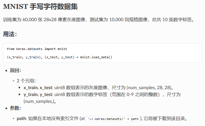
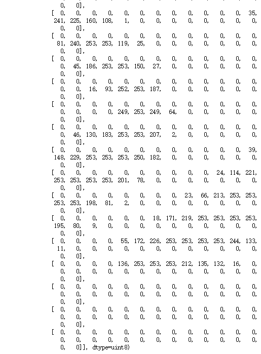
输入网络的数据X_train是60000张尺寸为28*28（共784个像素）的图像，对应y_train是秩为1的数组(60000, )

2.预处理数据

# data pre-processing
X_train = X_train.reshape(X_train.shape[0], -1) / 255.   # normalize
X_test = X_test.reshape(X_test.shape[0], -1) / 255.      # normalize
y_train = np_utils.to_categorical(y_train, num_classes=10)
y_test = np_utils.to_categorical(y_test, num_classes=10)

X_train = X_train.reshape(X_train.shape[0], -1) ，
将X_train展开成 60000x784 的形式，reshape里面的 -1相当于自适应行数或列数，这里 (60000x28x28) / 60000 =784，输入的 x 变成 60,000*784 的数据，然后除以 255 进行标准化，因为每个像素都是在 0 到 255 之间的，标准化之后就变成了 0 到 1 之间。

对于 y，要用到 Keras 改造的 numpy 的一个函数 np_utils.to_categorical，把 y 变成了 one-hot 的形式，即之前 y 是一个数值， 在 0-9 之间，现在是一个大小为 10 的向量，它属于哪个数字，就在哪个位置为 1，其他位置都是 0。

numpy.reshape( ,-1)

戳：numpy.reshape

这里直接搬运一个Example过来

>>> a = np.array([[1,2,3], [4,5,6]])
>>> np.reshape(a, 6)
array([1, 2, 3, 4, 5, 6])
>>> np.reshape(a, 6, order='F')
array([1, 4, 2, 5, 3, 6])
>>> np.reshape(a, (3,-1))       # the unspecified value is inferred to be 2
array([[1, 2],
       [3, 4],
       [5, 6]])

reshape里面的-1相当于自适应行数和列数，由python通过a和其他已知的维度值推测出来未定义的这个维度，再举个栗子

# 下面是两张2*3大小的照片
>>> image = np.array([[[1,2,3], [4,5,6]], [[1,1,1], [1,1,1]]])
>>> image.shape
(2, 2, 3)
# 假设不知道有几张照片，用-1代替，如何把所有二维照片给摊平成一维
>>> image.reshape((-1, 6))
array([[1, 2, 3, 4, 5, 6],
       [1, 1, 1, 1, 1, 1]])

独热编码(One-Hot Encoding)

在很多机器学习任务中，特征并不总是连续值，而有可能是分类值，离散特征的编码分为两种情况：

• 离散特征（分类变量）具有自然的有序关系（取值有大小的意义），比如size:[X,XL,XXL],那么就使用整数值的映射{X:1,XL:2,XXL:3}

• 离散特征（分类变量）之间不存在序数关系（取值之间没有大小的意义），比如color：[red,green,blue]，那么就使用独热编码(One-Hot Encoding)

独热编码又称一位有效编码。首先将分类值映射到整数值，然后把每个整数值表示为二进制向量，除了整数的索引（用1标记）之外，其它都是零值。

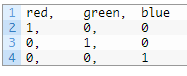
假设我们有一系列标签，其值为“红色”，“绿色”，“蓝色”。我们可以将’red’指定为整数值0，将’green’指定为整数值1，'bule’指定为2；只要我们总是将这些数字指定给这些标签，就称为整数编码。特征和对应编码需要保持一致，以便我们可以反编码，从整数值推出标签，实现对分类的预测。

接下来，我们可以创建一个二进制向量来表示每个整数值。对于3个可能的整数值，向量的长度为3。编码为0的“红色”标签将用二进制向量[1,0,0]表示，其中第0个索引标记为唯一的1值；编码为1的“绿色”标签将用二进制向量[0,1,0]，其中第1个索引标记为值1；编码为2的“蓝色”将用二进制向量[0,0,1]，其中第2个索引标记为值1。如下图所示：

One Hot Encode with scikit-learn
在此示例中，我们假设您具有以下3个标签的输出序列：

"cold"
"warm"
"hot"

10个时间步长的示例序列可以是：

cold, cold, warm, cold, hot, hot, warm, cold, warm, hot

这将首先需要整数编码，例如1,2,3。接下来是独热编码，由整数值到三位的二进制向量，例如[1,0,0]。

该序列提供序列中每个可能值的至少一个示例。因此，我们可以使用自动方法来定义标签到整数和整数到二进制向量的映射。

在这个例子中，我们将使用scikit-learn库中的编码器。具体来说，LabelEncoder用于创建标签的整数编码，OneHotEncoder用于创建整数编码值的独热编码。

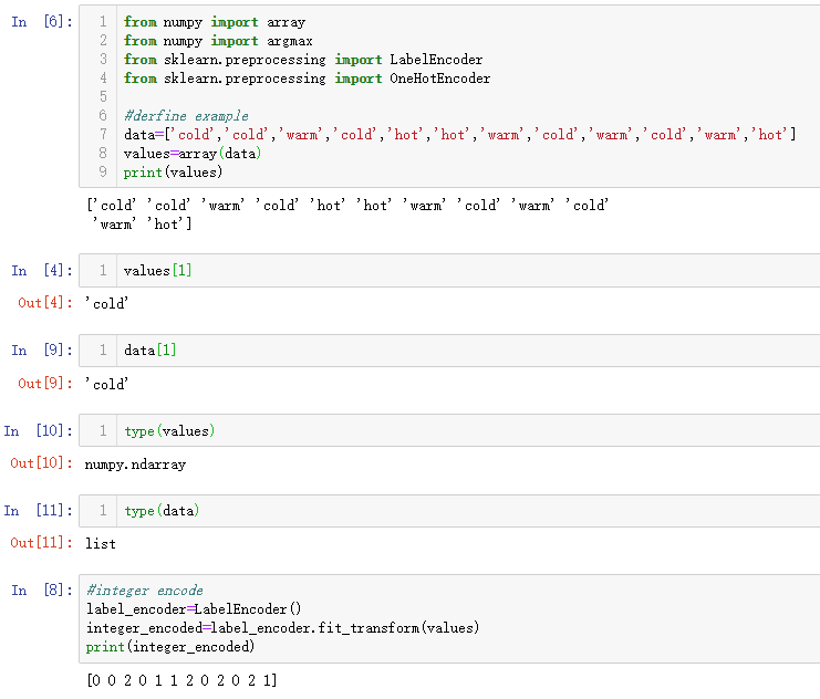
from numpy import array
from numpy import argmax
from sklearn.preprocessing import LabelEncoder
from sklearn.preprocessing import OneHotEncoder
# define example
data = ['cold', 'cold', 'warm', 'cold', 'hot', 'hot', 'warm', 'cold', 'warm', 'hot']
values = array(data)
print(values)
# integer encode
label_encoder = LabelEncoder()
integer_encoded = label_encoder.fit_transform(values)
print(integer_encoded)
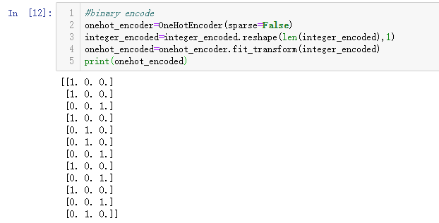
# binary encode
onehot_encoder = OneHotEncoder(sparse=False)
integer_encoded = integer_encoded.reshape(len(integer_encoded), 1)
onehot_encoded = onehot_encoder.fit_transform(integer_encoded)
print(onehot_encoded)
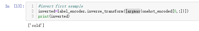
# invert first example
inverted = label_encoder.inverse_transform([argmax(onehot_encoded[0, :])])
print(inverted)

训练数据包含所有可能示例的集合，因此我们可以依赖整数和独热编码变换来创建标签到编码的完整映射。默认情况下，OneHotEncoder类将返回更有效的稀疏编码。这可能不适合某些应用程序，例如与Keras深度学习库一起使用。在这种情况下，我们通过设置sparse = False参数来禁用稀疏返回类型。

我们可以从这个3值的独热编码中得到预测，然后反变换为原始标签：使用Numpy.argmax函数来定位具有最大值的列的索引；然后将其馈送到LabelEncoder以计算反向变换，返回文本标签。

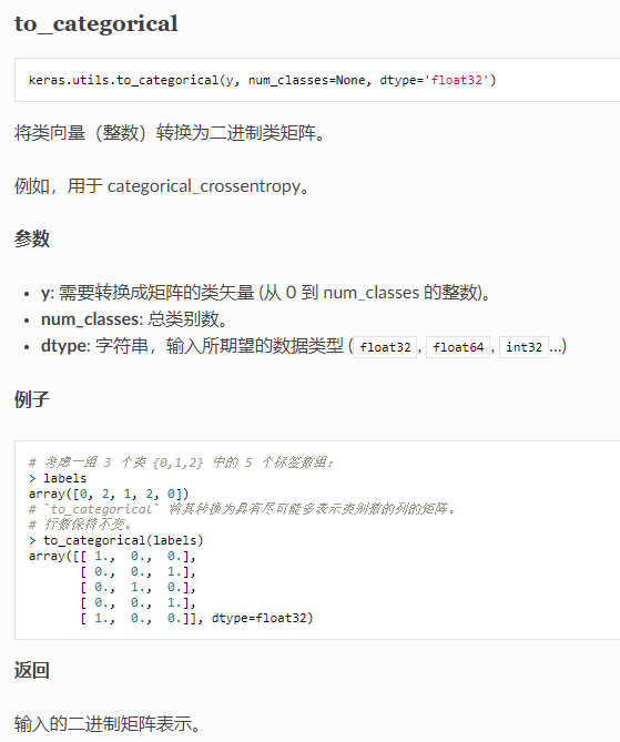
np_utils.to_categorical()

如果你有一个已经整数编码的序列，你可以直接使用整数编码（进行一些缩放之后）；如果整数之间没有真正的序数关系，实际上只是标签的占位符，那么可以直接对整数值进行独热编码，Keras库提供了一个名为to_categorical的函数来实现整数数值的独热编码。

3.创建模型

在上一篇搭建Regression神经网络的例子中，我们采用了先实例化Sequential()再通过.add()的方法把各层layers依次添加到模型中；这次采用第二种创建Sequential()模型的方法，把layers实例的列表传递给Sequential构造器，直接在模型里面加多个神经层；就像一个水管，一段一段的，数据是从上面一段掉到下面一段，再掉到下面一段。

# model=Sequential()
# model.add(...)

# Another way to build your neural net
model=Sequential([
    Dense(32,input_dim=784),
    Activation('relu'),
    Dense(10),
    Activation('softmax')
    ])

第一段就是加入 Dense 神经层，32是output_dim，也就是说，输入的784（input_dim）个数据通过这段“水管”之后，传出来的数据只有32个features，然后把这32个features传给激励单元，这里用relu作为Activation函数，这一步就是把它变成了非线性的数据。然后再经过一个Dense layer，输出10个单位(这一步不需要定义input_dim，因为它接收的是上一层的输出）。输出的10个单位需要放到10个class里面，所以最后再经过Activation layer的softmax函数进行分类。总结一下就是784个数据经过dense layer压缩为32个features，activation用的relu，再经过dense layer压缩为10个features，activation用的softmax进行分类处理。

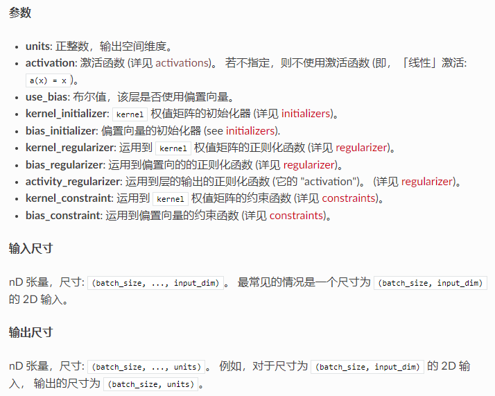
全连接层（Dense）

Dense 实现以下操作： output = activation(dot(input, kernel) + bias) 其中 activation 是按逐个元素计算的激活函数，kernel 是由网络层创建的权值矩阵，以及 bias 是其创建的偏置向量 (只在 use_bias 为 True 时才有用)。

• 注意: 如果该层的输入的秩大于2，那么它首先被展平然后 再计算与 kernel 的点乘。

# 作为 Sequential 模型的第一层
model = Sequential()
model.add(Dense(32, input_shape=(16,)))
# 现在模型就会以尺寸为 (*, 16) 的数组作为输入，
# 其输出数组的尺寸为 (*, 32)

# 在第一层之后，你就不再需要指定输入的尺寸了：
model.add(Dense(32))

keras.layers.Dense(units, activation=None, use_bias=True, kernel_initializer='glorot_uniform', bias_initializer='zeros', kernel_regularizer=None, bias_regularizer=None, activity_regularizer=None, kernel_constraint=None, bias_constraint=None)

激活函数（Activation）

激活函数是为了解决我们日常生活中，不能用线性方程所概括的问题，通过强行把原有的线性结果给扭曲了.，使得输出结果 y 也有了非线性的特征。激活函数可以通过设置单独的激活层实现，也可以在构造层对象时通过传递 activation 参数实现

from keras.layers import Activation, Dense

model.add(Dense(64))
model.add(Activation('tanh'))

等价于：

model.add(Dense(64, activation='tanh'))

你也可以通过传递一个逐元素运算的 Theano/TensorFlow/CNTK 函数来作为激活函数：

from keras import backend as K

model.add(Dense(64, activation=K.tanh))
model.add(Activation(K.tanh))

激励函数一定是可以微分的, 因为在 backpropagation 误差反向传递的时候, 只有这些可微分的激励函数才能把误差传递回去。 在少量层结构中, 我们可以尝试很多种不同的激励函数，在卷积神经网络 Convolutional neural networks 的卷积层中，推荐的激励函数是 relu；在循环神经网络中 recurrent neural networks，推荐的是 tanh 或者是 relu 。
 

4.激活模型

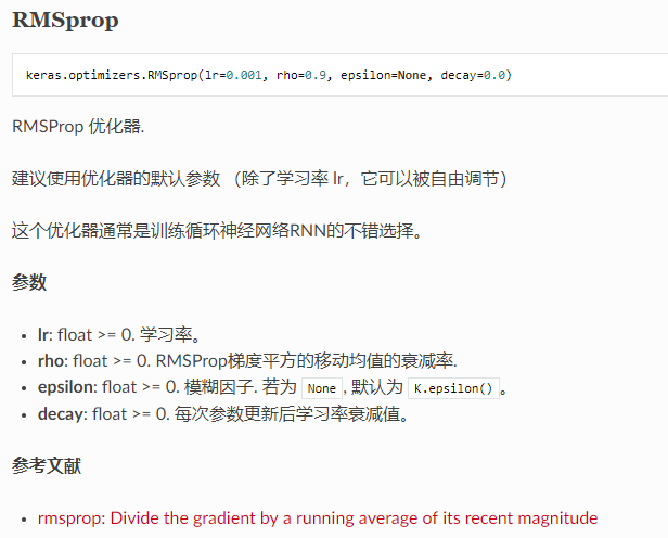
这里打算用rmsprop作为优化器（optimizer）更新我们的数据，参数包括学习率等。

# Another way to define your optimizer
rmsprop=RMSprop(lr=0.001,rho=0.9, epsilon=1e-08, decay=0.0)

定义好optimizer之后就可以配置模型了，用model.compile 激励我们的神经网络

# We add metrics to get more results you want to see
model.compile(
     optimizer=rmsprop,
     loss='categorical_crossentropy',
     metrics=['accuracy']
)

优化器，可以是默认的，也可以是我们在上一步定义的。 损失函数，分类和回归问题的不一样，分类这里用的是交叉熵，通过计算它的cross entropy来minimize loss。 metrics，在训练和测试期间的模型评估标准，里面可以放入需要计算的 cost，accuracy，score 等，在训练阶段会同时输出compile里的这些参数，在测试阶段也会计算这些参数，然后print输出查看。

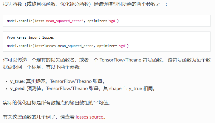
优化器 （optimzer）

优化器 (optimizer) 是编译 Keras 模型的所需的两个参数之一：

from keras import optimizers

model = Sequential()
model.add(Dense(64, kernel_initializer='uniform', input_shape=(10,)))
model.add(Activation('softmax'))

sgd = optimizers.SGD(lr=0.01, decay=1e-6, momentum=0.9, nesterov=True)
model.compile(loss='mean_squared_error', optimizer=sgd)

你可以先实例化一个优化器对象，然后将它传入 model.compile()，像上述示例中一样， 或者你可以通过名称来调用优化器。在后一种情况下，将使用优化器的默认参数。

# 传入优化器名称: 默认参数将被采用
model.compile(loss='mean_squared_error', optimizer='sgd')

损失函数 （Losses）

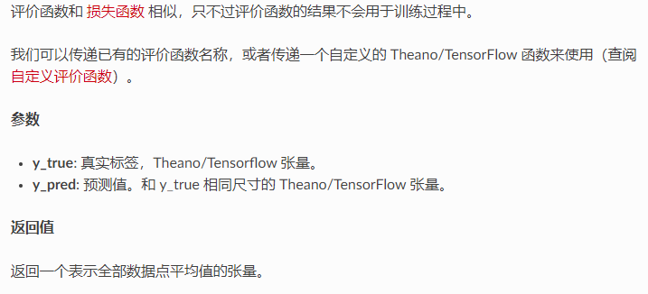
评价函数（Metrics）

评价函数用于评估当前训练模型的性能。当模型编译后（compile），评价函数应该作为 metrics 的参数来输入。

model.compile(loss='mean_squared_error',
              optimizer='sgd',
              metrics=['mae', 'acc'])

from keras import metrics

model.compile(loss='mean_squared_error',
              optimizer='sgd',
              metrics=[metrics.mae, metrics.categorical_accuracy])

5.训练模型

这里用的是model.fit，以固定数量的轮次（数据集上的迭代）训练模型，返回一个 History 对象，其 History.history 属性是连续 epoch 训练损失和评估值，以及验证集损失和评估值的记录（如果设置了验证集）

model.fit(X_train,y_train,nb_epoch=2,batch_size=32)

• batch_size: 每次梯度更新的样本数，如果未指定，默认为 32。
• epochs: 训练模型迭代轮次。一个轮次是在整个 x 或 y 上的一轮迭代。请注意，与 initial_epoch 一起，epochs被理解为 「最终轮次」。模型并不是训练了 epochs 轮，而是到第 epochs 轮停止训练。
• validation_split: 在 0 和 1 之间浮动。用作验证集的训练数据的比例。并将在每一轮结束时评估这些验证数据的误差和任何其他模型指标。
• validation_data: 元组 (x_val，y_val) 或元组 (x_val，y_val，val_sample_weights)，用来评估损失，以及在每轮结束时的任何模型度量指标。模型将不会在这个数据上进行训练。这个参数会覆盖 validation_split。

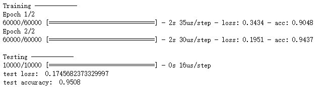
6.测试模型

用测试集来检验一下模型，model.evaluate返回误差值和评估标准值，计算逐批次进行。运行代码之后，可以输出 accuracy 和 loss （model.compile里设置的）

# Evaluate the model with the metrics we defined earlier
loss, accuracy = model.evaluate(X_test, y_test)

print('test loss: ', loss)
print('test accuracy: ', accuracy)

参考

莫烦Keras-Classifier 分类
Keras Documentation

How to One Hot Encode Sequence Data in Python
OneHotEncoder scikit-learn API documentation
LabelEncoder scikit-learn API documentation
to_categorical Keras API文档