


参照《机器学习实战》第二版
本章探讨的大部分主题对于理解、构建和训练神经网络是至关重要的。
目的在于了解系统是如何工作的,它有助于快速定位到适合的模型、正确的训练算法,以及一套合适的参数。不仅如此,后期还能让你更高效的执行错误调试和错误分析。
我们将从最简单的模型之一 – 线性回归模型开始,介绍两种非常不同的训练模型的方法:
- 通过
“闭式”方程,直接计算出最拟合训练集的模型参数(也就是使训练集上的成本模型最小化的模型参数)。 - 使用
迭代优化的方法,即梯度下降(GD),逐渐调整模型参数直至训练集上的成本函数调至最低,最终趋于第一种方法计算出来模型参数。我们还会研究几个梯度下降的变体,包括批量梯度下降、小批量梯度下降以及随机梯度下降。
接着我们进入多项式回归的讨论,这是一个更为复杂的模型,更适合非线性数据集。由于该模型的参数比线性模型更多,因此更容易对训练数据过拟合,我们将使用学习曲线来分辨这种情况是否发生。然后,再介绍几种正则化技巧,降低过拟合训练数据的风险。
最后,我们将学习两种经常用于分来任务的模型:Logistic回归和Softmax回归。
1、线性回归
1.1、公式:线性回归模型预测
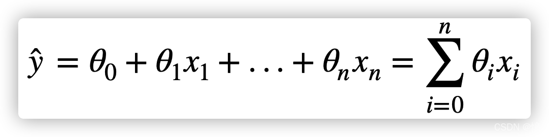
- y ^ \hat{y} y^:是预测值
- n n n:是特征数i
- x i x_i xi:是第 i 个特征值
- θ j \theta_j θj:是第 j 个模型参数
1.2、公式:线性回归模型预测(向量化形式)
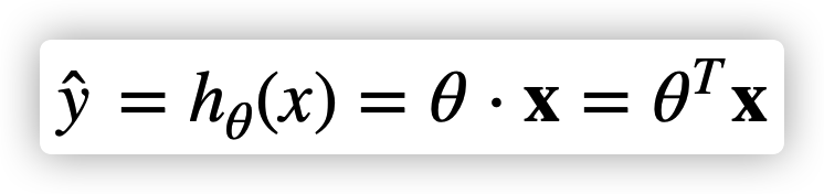
- θ ⃗ \vec\theta θ:是模型的参数向量
- x ⃗ \vec{x} x:是实例的特征向量
- θ ⃗ ⋅ x ⃗ \vec\theta \cdot \vec{x} θ⋅x:是两个向量的点积
- h θ h_\theta hθ:是假设函数,使用模型参数 θ ⃗ \vec\theta θ
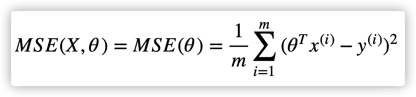
1.3、公式:线性回归模型的 MSE 成本函数
回归模型常见的性能指标是均方根误差(RMSE)。因此,在训练线性回归模型时,你需要找到最小化 RMSE 的
θ
⃗
\vec\theta
θ 值。在实践中,最小化均方误差(MSE)比最小化均方根误差(RMSE)更为简单,两者效果相同(因为使函数最小的值,同样也使其平方根最小)。
在训练集 X 上,使用该公式计算训练集 X 上线性回归的 MSE,
h
θ
h_\theta
hθ为假设函数:
1.4、公式:标准方程
为了得到是成本方程最小的
θ
\theta
θ 值,有个闭式解方法 – 也就是直接得出结果数学方程,即标准方程:
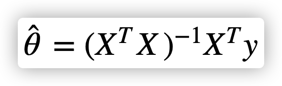
- θ ⃗ ^ \hat{\vec\theta} θ^:是使成本函数最小的值
- y y y:是包含 y ( 1 ) y^{(1)} y(1)到 y ( m ) y^{(m)} y(m)的目标值向量
1.5、测试上面公式
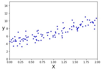
随机生成一些线性数据来测试上面公式:
import numpy as np

np.random.seed(42)
X = np.random.rand(100, 1) * 2
y = 4 + 3 * X + np.random.randn(100, 1)
import matplotlib.pyplot as plt

plt.plot(X, y, "b.")
plt.xlabel("X", fontsize=18)
plt.ylabel("y", rotation=0, fontsize=18)
plt.axis([0, 2, 0, 15])
plt.show()
现在使用标准方程来计算
θ
⃗
^
\hat{\vec\theta}
θ^。使用NumPy的线性代数模块np.linalg中的inv()函数来对矩阵求逆,并利用dot()函数计算矩阵的内积:
X_b = np.c_[np.ones((100, 1)), X]
theta_best = np.linalg.inv(X_b.T.dot(X_b)).dot(X_b.T).dot(y)
theta_best  # MSE 成本方程最小值
array([[4.21509616],
       [2.77011339]])
根据我们上面y的公式,我们可以知道,我们所期望的
θ
0
=
4
\theta_0 = 4
θ0=4,
θ
1
=
3
\theta_1 = 3
θ1=3,而得到的却是
θ
0
=
4.215
\theta_0 = 4.215
θ0=4.215,
θ
1
=
2.770
\theta_1 = 2.770
θ1=2.770,这是因为有噪声的存在,导致无法完全还原原本的函数。
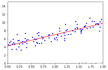
现在可以使用 θ ^ \hat{\theta} θ^做出预测:
X_new = np.array([[0], [2]])
X_new_b = np.c_[np.ones((2, 1)), X_new]
y_predict = X_new_b.dot(theta_best)
y_predict  # 预测两个x值的y
array([[4.21509616],
       [9.75532293]])
plt.plot(X, y, "b.")
plt.plot(X_new, y_predict, "r-")
plt.axis([0, 2, 0, 15])
plt.show()
1.6、Scikit-Learn 方法
from sklearn.linear_model import LinearRegression

lin_reg = LinearRegression()
lin_reg.fit(X, y)
lin_reg.intercept_, lin_reg.coef_
(array([4.21509616]), array([[2.77011339]]))
lin_reg.predict(X_new)
array([[4.21509616],
       [9.75532293]])
LinearRegression类基于scipy.linalg.lstsq()函数(即最小二乘法),可以直接调用:
theta_best_svd, residuals, rank, s = np.linalg.lstsq(X_b, y, rcond=1e-6)
theta_best_svd
array([[4.21509616],
       [2.77011339]])
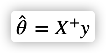
此处计算公式为
θ
^
=
X
+
y
\hat{\theta} = X^{+}y
θ^=X+y,其中
X
+
X^{+}
X+ 是
X
X
X 的伪逆。可以直接使用np.linalg.pinv()来直接计算这个伪逆:
伪逆本身是使用被成为奇异值分解(SVD)的标准矩阵分解技术来计算的。
np.linalg.pinv(X_b).dot(y)
array([[4.21509616],
       [2.77011339]])
1.7、计算复杂度
标准方程计算
X
T
X
X^TX
XTX 的逆,
X
T
X
X^TX
XTX 是一个(n+1)×(n+1)的矩阵(n是特征向量)。这种矩阵求逆的计算复杂度通常为
O
(
n
2.4
)
O(n^{2.4})
O(n2.4) 到
O
(
n
3
)
O(n^3)
O(n3),取决于具体现实。换句话说,如果将特征数量翻倍,那么计算时间将乘以大约
2
2.4
=
5.3
2^{2.4}=5.3
22.4=5.3倍 到
2
3
=
8
2^3=8
23=8倍。
Scikit-Learn的LinearRegression类使用的SVD方法的复杂度约为
O
(
n
2
)
O(n^2)
O(n2)。即特征数量翻倍,计算时间大约是原来的 4 倍。
2、梯度下降
2.1、批量梯度下降
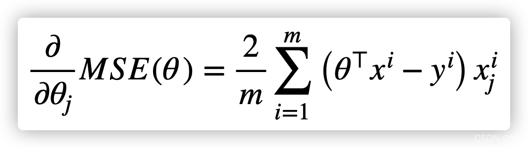
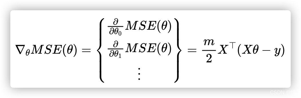
要实现梯度下降,你需要计算每个模型关于参数
θ
j
\theta_j
θj 的成本函数梯度。换言之,就是关于
θ
j
\theta_j
θj 的偏导数:
- 公式:
- 公式(向量化):
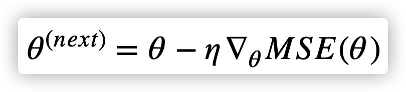
一旦有了梯度向量,从 θ \theta θ 中减去 ∇ θ M S E ( θ ) \nabla_{\theta} MSE(\theta) ∇θMSE(θ) 。这时候学习率 η 就发挥作用了:用梯度向量乘以 η 确定下坡步长的大小:
算法实现:
eta = 0.1  # 学习率
n_iterations = 1000  # 梯度下降次数
m = len(X)  # 100个实例,X的数量
s = {}

theta = np.random.rand(2, 1)
s[0] = "{} {}".format(theta[0], theta[1])
for iteration in range(n_iterations):
    gradients = 2/m * X_b.T.dot(X_b.dot(theta) - y)
    theta = theta - eta * gradients
    s[iteration + 1] = "({:>2}){} {}\t-> {} {}".format(iteration, gradients[0], gradients[1], theta[0], theta[1])
theta
array([[4.21509616],
       [2.77011339]])
X_new_b.dot(theta)
array([[4.21509616],
       [9.75532293]])
# 显示前几次的运算结果
for i in range(20):
    print(s[i])
[0.7948113] [0.50263709]
( 0)[-11.10506446] [-12.03209351]	-> [1.90531775] [1.70584644]
( 1)[-6.6211481] [-6.97223824]	-> [2.56743256] [2.40307027]
( 2)[-3.98563362] [-4.00520407]	-> [2.96599592] [2.80359067]
( 3)[-2.43523896] [-2.26654005]	-> [3.20951982] [3.03024468]
( 4)[-1.52191778] [-1.24882174]	-> [3.3617116] [3.15512685]
( 5)[-0.98266545] [-0.65419726]	-> [3.45997814] [3.22054658]
( 6)[-0.66309598] [-0.30783247]	-> [3.52628774] [3.25132983]
( 7)[-0.47258202] [-0.1071039]	-> [3.57354594] [3.26204022]
( 8)[-0.35792234] [0.00822477]	-> [3.60933818] [3.26121774]
( 9)[-0.28788473] [0.07350896]	-> [3.63812665] [3.25386684]
(10)[-0.24413278] [0.10949922]	-> [3.66253993] [3.24291692]
(11)[-0.21589999] [0.12837323]	-> [3.68412993] [3.2300796]
(12)[-0.19686344] [0.13727654]	-> [3.70381627] [3.21635195]
(13)[-0.18330867] [0.14040094]	-> [3.72214714] [3.20231185]
(14)[-0.17305246] [0.14020451]	-> [3.73945238] [3.1882914]
(15)[-0.16481055] [0.13812767]	-> [3.75593344] [3.17447863]
(16)[-0.15782643] [0.13501363]	-> [3.77171608] [3.16097727]
(17)[-0.15165347] [0.13135508]	-> [3.78688143] [3.14784176]
(18)[-0.14602703] [0.12743903]	-> [3.80148413] [3.13509786]
theta_path_bgd = []

def plot_gradient_descent(theta, eta, theta_path=None):
    m = len(X_b)
    plt.plot(X, y, "b.")
    n_iterations = 1000
    for iteration in range(n_iterations):
        if iteration < 10:  # 画出前十条线
            y_predict = X_new_b.dot(theta)
            style = "b-" if iteration > 0 else "r--"  # 第一条线是红色虚线,其余是蓝色实线
            plt.plot(X_new, y_predict, style)
        gradients = 2/m * X_b.T.dot(X_b.dot(theta) - y)
        theta = theta - eta * gradients
        if theta_path is not None:
            theta_path.append(theta)

    plt.xlabel("$x_1$", fontsize=18)
    plt.axis([0, 2, 0, 15])
    plt.title(r"$\eta = {}$".format(eta), fontsize=16)
np.random.seed(42)
theta = np.random.randn(2,1)
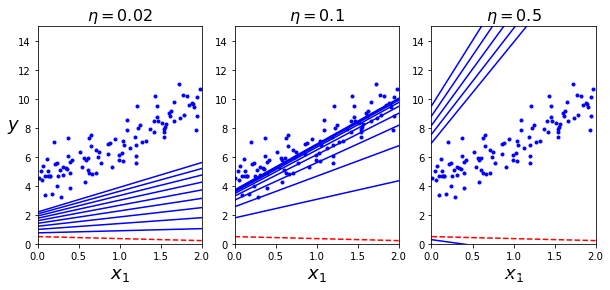
plt.figure(figsize=(10,4))
plt.subplot(131); plot_gradient_descent(theta, eta=0.02)
plt.ylabel("$y$", rotation=0, fontsize=18)
plt.subplot(132); plot_gradient_descent(theta, eta=0.1, theta_path=theta_path_bgd)
plt.subplot(133); plot_gradient_descent(theta, eta=0.5)
plt.show()
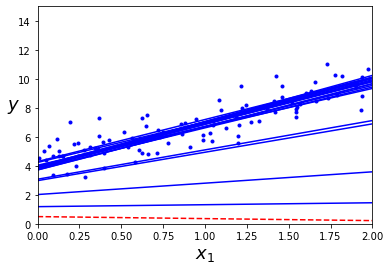
2.2、随机梯度下降
优点在于快,每次随机挑选一个实例用于计算(而不是 全部实例计算)。
np.random.seed(42)
theta_path_sgd = []

m = len(X_b)
n_epochs = 50   # 梯度下降次数
t0, t1 = 5, 50  # 学习进度超参数
s = dict()

def learning_schedule(t):
    """ 学习计划 """
    return t0 / (t + t1)

theta = np.random.randn(2,1)  # 随机初始化
s[0] = "{} {}".format(theta[0], theta[1])
for epoch in range(n_epochs):
    for i in range(m):
        if epoch == 0 and i < 20:  # 只画出前20条线
            y_predict = X_new_b.dot(theta)
            style = "b-" if i > 0 else "r--"
            plt.plot(X_new, y_predict, style)
        random_index = np.random.randint(m)
        xi = X_b[random_index:random_index+1]  # 随机取出一个实例的 x
        yi = y[random_index:random_index+1]    # 随机取出一个实例的 y
        gradients = 2 * xi.T.dot(xi.dot(theta) - yi)
        eta = learning_schedule(epoch * m + i) # 减小梯度
        theta = theta - eta * gradients
        theta_path_sgd.append(theta)
        s[epoch * m + i + 1] = "({}, {:>2} -> {:.5f}){} {}\t-> {} {}".format(epoch, i, eta, gradients[0], gradients[1], theta[0], theta[1])

plt.plot(X, y, "b.")
plt.xlabel("$x_1$", fontsize=18)
plt.ylabel("$y$", rotation=0, fontsize=18)
plt.axis([0, 2, 0, 15])

plt.show()
theta
array([[4.21076011],
       [2.74856079]])
X_new_b.dot(theta)
array([[4.21076011],
       [9.7078817 ]])
# 显示前20次的运算结果
for i in range(20):
    print(s[i])
[0.49671415] [-0.1382643]
(0,  0 -> 0.10000)[-6.86014779] [-2.72643789]	-> [1.18272893] [0.13437949]
(0,  1 -> 0.09804)[-8.52324201] [-6.62558121]	-> [2.01834089] [0.78394627]
(0,  2 -> 0.09615)[-9.97915432] [-12.21154892]	-> [2.97787496] [1.95813367]
(0,  3 -> 0.09434)[-1.04064913] [-0.68869748]	-> [3.07604941] [2.02310513]
(0,  4 -> 0.09259)[-7.01608648] [-10.23796008]	-> [3.72568705] [2.9710644]
(0,  5 -> 0.09091)[-1.13142499] [-1.59951213]	-> [3.82854386] [3.11647459]
(0,  6 -> 0.08929)[-0.5145743] [-0.72746125]	-> [3.874488] [3.18142649]
(0,  7 -> 0.08772)[1.85301988] [2.36281333]	-> [3.71194239] [2.97416216]
(0,  8 -> 0.08621)[-2.24163244] [-0.48370585]	-> [3.90518657] [3.01586094]
(0,  9 -> 0.08475)[0.30279077] [0.22186197]	-> [3.87952633] [2.99705908]
(0, 10 -> 0.08333)[-0.43307984] [-0.63402364]	-> [3.91561632] [3.04989438]
(0, 11 -> 0.08197)[-0.66303807] [-0.18497948]	-> [3.9699637] [3.06505663]
(0, 12 -> 0.08065)[-0.01489278] [-0.0279835]	-> [3.97116473] [3.06731337]
(0, 13 -> 0.07937)[0.79632729] [1.51415949]	-> [3.90796416] [2.94714198]
(0, 14 -> 0.07812)[1.32249284] [1.68633038]	-> [3.8046444] [2.81539742]
(0, 15 -> 0.07692)[-1.23311237] [-0.11455716]	-> [3.8994992] [2.82420951]
(0, 16 -> 0.07576)[-5.19616514] [-1.01504087]	-> [4.29314807] [2.90110654]
(0, 17 -> 0.07463)[0.80823315] [1.53679763]	-> [4.23283217] [2.78642015]
(0, 18 -> 0.07353)[2.62261168] [1.87125088]	-> [4.03999307] [2.64882817]
2.3、小批量梯度下降
小批量梯度下降优于随机梯度下降的主要优点是,你可以通过矩阵操作的硬件优化来提高性能,特别是在使用GPU时。
theta_path_mgd = []

n_iterations = 50
minibatch_size = 20
s = dict()

np.random.seed(42)
theta = np.random.randn(2,1)

t0, t1 = 200, 1000
def learning_schedule(t):
    return t0 / (t + t1)

t = 0
s[0] = "{} {}".format(theta[0], theta[1])
for epoch in range(n_iterations):
    shuffled_indices = np.random.permutation(m)
    X_b_shuffled = X_b[shuffled_indices]
    y_shuffled = y[shuffled_indices]
    for i in range(0, m, minibatch_size):
        t += 1
        xi = X_b_shuffled[i:i+minibatch_size]
        yi = y_shuffled[i:i+minibatch_size]
        gradients = 2/minibatch_size * xi.T.dot(xi.dot(theta) - yi)
        eta = learning_schedule(t)
        theta = theta - eta * gradients
        theta_path_mgd.append(theta)
        s[t] = "({}, {:>2} -> {:.5f}){} {}\t-> {} {}".format(epoch, i, eta, gradients[0], gradients[1], theta[0], theta[1])
theta
array([[4.25214635],
       [2.7896408 ]])
# 显示前20次的运算结果
for i in range(20):
    print(s[i])
[0.49671415] [-0.1382643]
(0,  0 -> 0.19980)[-13.79245989] [-16.28677942]	-> [3.25245039] [3.11583748]
(0, 20 -> 0.19960)[-1.60389476] [-1.03975953]	-> [3.57258907] [3.32337431]
(0, 40 -> 0.19940)[0.69601284] [0.98286925]	-> [3.43380286] [3.12738842]
(0, 60 -> 0.19920)[-1.07936129] [-0.37991824]	-> [3.64881507] [3.20306935]
(0, 80 -> 0.19900)[-0.32903101] [-0.00213246]	-> [3.71429388] [3.20349372]
(1,  0 -> 0.19881)[-0.64125174] [-0.2601402]	-> [3.84177931] [3.25521145]
(1, 20 -> 0.19861)[0.34496049] [0.39959046]	-> [3.7732668] [3.1758489]
(1, 40 -> 0.19841)[-0.41821607] [-0.17210907]	-> [3.85624618] [3.20999752]
(1, 60 -> 0.19822)[0.48598075] [1.058177]	-> [3.759917] [3.00024985]
(1, 80 -> 0.19802)[-0.29018363] [-0.16202744]	-> [3.8173791] [3.03233449]
(2,  0 -> 0.19782)[-0.56934643] [-0.1323744]	-> [3.93000945] [3.05852132]
(2, 20 -> 0.19763)[0.56698072] [0.62460951]	-> [3.81795793] [2.9350807]
(2, 40 -> 0.19743)[-0.60787495] [-0.14207289]	-> [3.93797273] [2.96313063]
(2, 60 -> 0.19724)[0.06525087] [0.0170397]	-> [3.92510273] [2.95976974]
(2, 80 -> 0.19704)[-0.65616741] [-0.64608421]	-> [4.0543968] [3.08707698]
(3,  0 -> 0.19685)[0.37921206] [0.60912079]	-> [3.97974876] [2.96717131]
(3, 20 -> 0.19666)[-0.5824764] [-0.59470588]	-> [4.09429672] [3.08412429]
(3, 40 -> 0.19646)[0.19575307] [0.36578361]	-> [4.05583836] [3.0122611]
(3, 60 -> 0.19627)[0.20283418] [0.37892469]	-> [4.01602792] [2.93788923]
theta_path_bgd = np.array(theta_path_bgd)
theta_path_sgd = np.array(theta_path_sgd)
theta_path_mgd = np.array(theta_path_mgd)
plt.figure(figsize=(14,8))
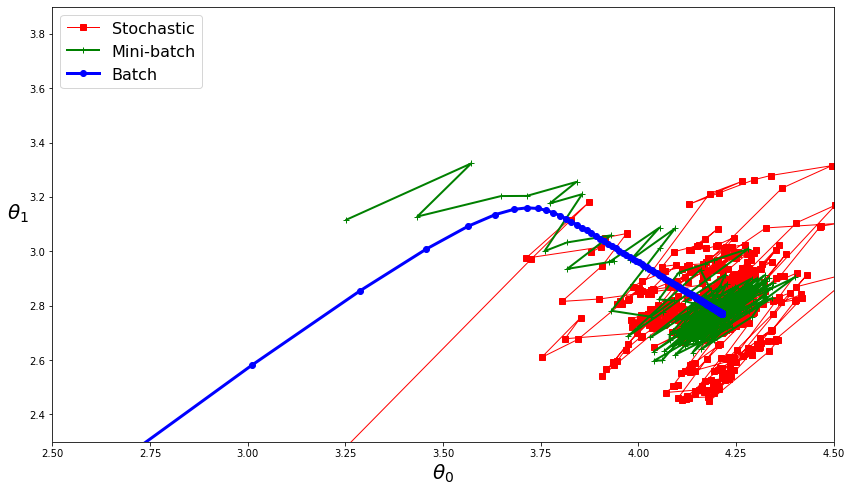
plt.plot(theta_path_sgd[:, 0], theta_path_sgd[:, 1], "r-s", linewidth=1, label="Stochastic") # 随机批量梯度下降
plt.plot(theta_path_mgd[:, 0], theta_path_mgd[:, 1], "g-+", linewidth=2, label="Mini-batch") # 小随机梯度下降
plt.plot(theta_path_bgd[:, 0], theta_path_bgd[:, 1], "b-o", linewidth=3, label="Batch") # 批量梯度下降
plt.legend(loc="upper left", fontsize=16)
plt.xlabel(r"$\theta_0$", fontsize=20)
plt.ylabel(r"$\theta_1$ ", fontsize=20, rotation=0)
plt.axis([2.5, 4.5, 2.3, 3.9])
plt.show()
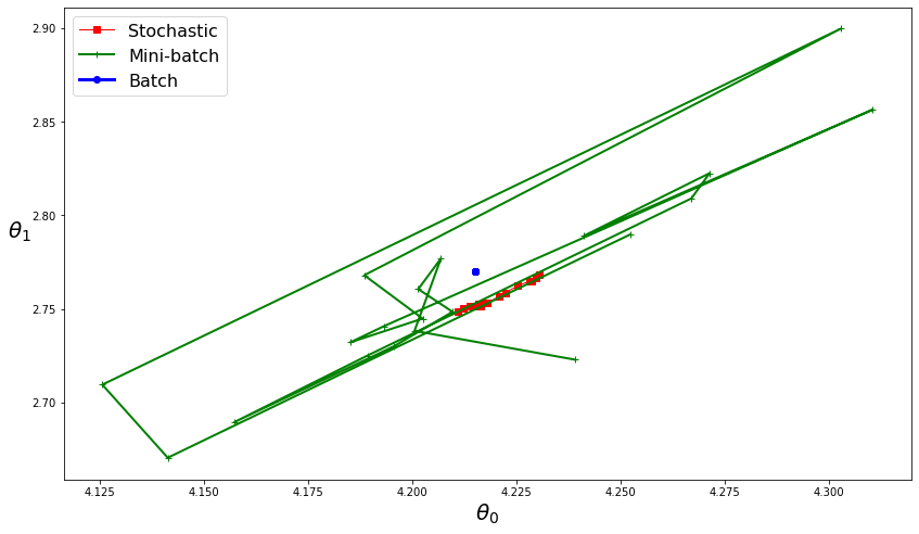
# 最后20次
plt.figure(figsize=(14,8))
plt.plot(theta_path_sgd[-20:, 0], theta_path_sgd[-20:, 1], "r-s", linewidth=1, label="Stochastic")  # 随机批量梯度下降
plt.plot(theta_path_mgd[-20:, 0], theta_path_mgd[-20:, 1], "g-+", linewidth=2, label="Mini-batch")  # 小随机梯度下降
plt.plot(theta_path_bgd[-20:, 0], theta_path_bgd[-20:, 1], "b-o", linewidth=3, label="Batch")       # 批量梯度下降
plt.legend(loc="upper left", fontsize=16)
plt.xlabel(r"$\theta_0$", fontsize=20)
plt.ylabel(r"$\theta_1$   ", fontsize=20, rotation=0)
# plt.axis([2.5, 4.5, 2.3, 3.9])
plt.show()
上图可知,小批量梯度下降效果最好。
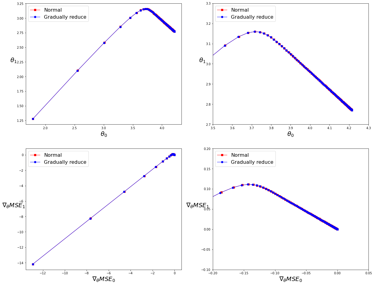
2.4、探索:批量梯度下降(学习率是否可变)
下面探索可以得知
- 当学习率在合理范围内,
学习率逐步降低对批量梯度下降没有太大影响。可以忽略不计。 - 当学习率在大于合理范围,
学习率逐步降低对批量梯度下降有影响,可以使学习率回归正常范围。
gradients_bgd_1 = []
theta_bgd_1 = []

def plot_gradient_descent_1(theta, eta, gradients_bgd, theta_bgd):
    """
    批量地梯度下降:正常
    """
    m = len(X)
    n_iterations = 1000
    for iteration in range(n_iterations):
        gradients = 2/m * X_b.T.dot(X_b.dot(theta) - y)
        theta = theta - eta * gradients
        gradients_bgd.append(gradients)
        theta_bgd.append(theta)
gradients_bgd_2 = []
theta_bgd_2 = []

def plot_gradient_descent_2(theta, t0, t1, gradients_bgd, theta_bgd):
    """
    批量地梯度下降:学习率逐步降低
    """
    t = 0
    m = len(X)
    n_iterations = t1
    minibatch_size = t0
    for epoch in range(n_iterations):
        for i in range(0, m, minibatch_size):
            t += 1
            gradients = 2/m * X_b.T.dot(X_b.dot(theta) - y)
            eta = t0 / (t + t1)
            theta = theta - eta * gradients
            gradients_bgd.append(gradients)
            theta_bgd.append(theta)
np.random.seed(42)
theta = np.random.randn(2,1)
plot_gradient_descent_1(theta, 0.1, gradients_bgd_1, theta_bgd_1)

np.random.seed(42)
theta = np.random.randn(2,1)
plot_gradient_descent_2(theta, 100, 1000, gradients_bgd_2, theta_bgd_2)
gradients_bgd_1 = np.array(gradients_bgd_1)
theta_bgd_1 = np.array(theta_bgd_1)
gradients_bgd_2 = np.array(gradients_bgd_2)
theta_bgd_2 = np.array(theta_bgd_2)
plt.figure(figsize=(20, 16))

plt.subplot(221);
plt.plot(theta_bgd_1[:, 0], theta_bgd_1[:, 1], "r-s", linewidth=1, label="Normal")            # 正常
plt.plot(theta_bgd_2[:, 0], theta_bgd_2[:, 1], "b-o", linewidth=1, label="Gradually reduce")  # 逐步降低学习率
plt.legend(loc="upper left", fontsize=16)
plt.xlabel(r"$\theta_0$", fontsize=20)
plt.ylabel(r"$\theta_1$   ", fontsize=20, rotation=0)

plt.subplot(222);
plt.plot(theta_bgd_1[:, 0], theta_bgd_1[:, 1], "r-s", linewidth=1, label="Normal")            # 正常
plt.plot(theta_bgd_2[:, 0], theta_bgd_2[:, 1], "b-o", linewidth=1, label="Gradually reduce")  # 逐步降低学习率
plt.legend(loc="upper left", fontsize=16)
plt.xlabel(r"$\theta_0$", fontsize=20)
plt.ylabel(r"$\theta_1$   ", fontsize=20, rotation=0)
plt.axis([3.5, 4.3, 2.7, 3.3])  # 放大

plt.subplot(223);
plt.plot(gradients_bgd_1[:, 0], gradients_bgd_1[:, 1], "r-s", linewidth=1, label="Normal")            # 正常
plt.plot(gradients_bgd_2[:, 0], gradients_bgd_2[:, 1], "b-o", linewidth=1, label="Gradually reduce")  # 逐步降低学习率
plt.legend(loc="upper left", fontsize=16)
plt.xlabel(r"$\nabla_{\theta} MSE_0$", fontsize=20)
plt.ylabel(r"$\nabla_{\theta} MSE_1$   ", fontsize=20, rotation=0)

plt.subplot(224);
plt.plot(gradients_bgd_1[:, 0], gradients_bgd_1[:, 1], "r-s", linewidth=1, label="Normal")            # 正常
plt.plot(gradients_bgd_2[:, 0], gradients_bgd_2[:, 1], "b-o", linewidth=1, label="Gradually reduce")  # 逐步降低学习率
plt.legend(loc="upper left", fontsize=16)
plt.xlabel(r"$\nabla_{\theta} MSE_0$", fontsize=20)
plt.ylabel(r"$\nabla_{\theta} MSE_1$   ", fontsize=20, rotation=0)
plt.axis([-0.2, 0.05, -0.1, 0.2])  # 放大

plt.show()
gradients_bgd_3 = []
theta_bgd_3 = []
np.random.seed(42)
theta = np.random.randn(2,1)
plot_gradient_descent_1(theta, 0.5, gradients_bgd_3, theta_bgd_3)

gradients_bgd_4 = []
theta_bgd_4 = []
np.random.seed(42)
theta = np.random.randn(2,1)
plot_gradient_descent_2(theta, 500, 1000, gradients_bgd_4, theta_bgd_4)
gradients_bgd_3 = np.array(gradients_bgd_3)
theta_bgd_3 = np.array(theta_bgd_3)
gradients_bgd_4 = np.array(gradients_bgd_4)
theta_bgd_4 = np.array(theta_bgd_4)
plt.figure(figsize=(20, 16))

plt.subplot(221);
plt.plot(theta_bgd_3[:, 0], theta_bgd_3[:, 1], "r-s", linewidth=1, label="Normal")            # 正常
plt.plot(theta_bgd_4[:, 0], theta_bgd_4[:, 1], "b-o", linewidth=1, label="Gradually reduce")  # 逐步降低学习率
plt.legend(loc="upper left", fontsize=16)
plt.xlabel(r"$\theta_0$", fontsize=20)
plt.ylabel(r"$\theta_1$   ", fontsize=20, rotation=0)

plt.subplot(222);
plt.plot(theta_bgd_3[:, 0], theta_bgd_3[:, 1], "r-s", linewidth=1, label="Normal")            # 正常
plt.plot(theta_bgd_4[:, 0], theta_bgd_4[:, 1], "b-o", linewidth=1, label="Gradually reduce")  # 逐步降低学习率
plt.legend(loc="upper left", fontsize=16)
plt.xlabel(r"$\theta_0$", fontsize=20)
plt.ylabel(r"$\theta_1$   ", fontsize=20, rotation=0)
plt.axis([4.1, 4.3, 2.7, 2.9])  # 放大

plt.subplot(223);
plt.plot(gradients_bgd_3[:, 0], gradients_bgd_3[:, 1], "r-s", linewidth=1, label="Normal")            # 正常
plt.plot(gradients_bgd_4[:, 0], gradients_bgd_4[:, 1], "b-o", linewidth=1, label="Gradually reduce")  # 逐步降低学习率
plt.legend(loc="upper left", fontsize=16)
plt.xlabel(r"$\nabla_{\theta} MSE_0$", fontsize=20)
plt.ylabel(r"$\nabla_{\theta} MSE_1$   ", fontsize=20, rotation=0)

plt.subplot(224);
plt.plot(gradients_bgd_3[:, 0], gradients_bgd_3[:, 1], "r-s", linewidth=1, label="Normal")            # 正常
plt.plot(gradients_bgd_4[:, 0], gradients_bgd_4[:, 1], "b-o", linewidth=1, label="Gradually reduce")  # 逐步降低学习率
plt.legend(loc="upper left", fontsize=16)
plt.xlabel(r"$\nabla_{\theta} MSE_0$", fontsize=20)
plt.ylabel(r"$\nabla_{\theta} MSE_1$   ", fontsize=20, rotation=0)
plt.axis([-0.15, 0.05, -0.1, 0.1])  # 放大

plt.show()
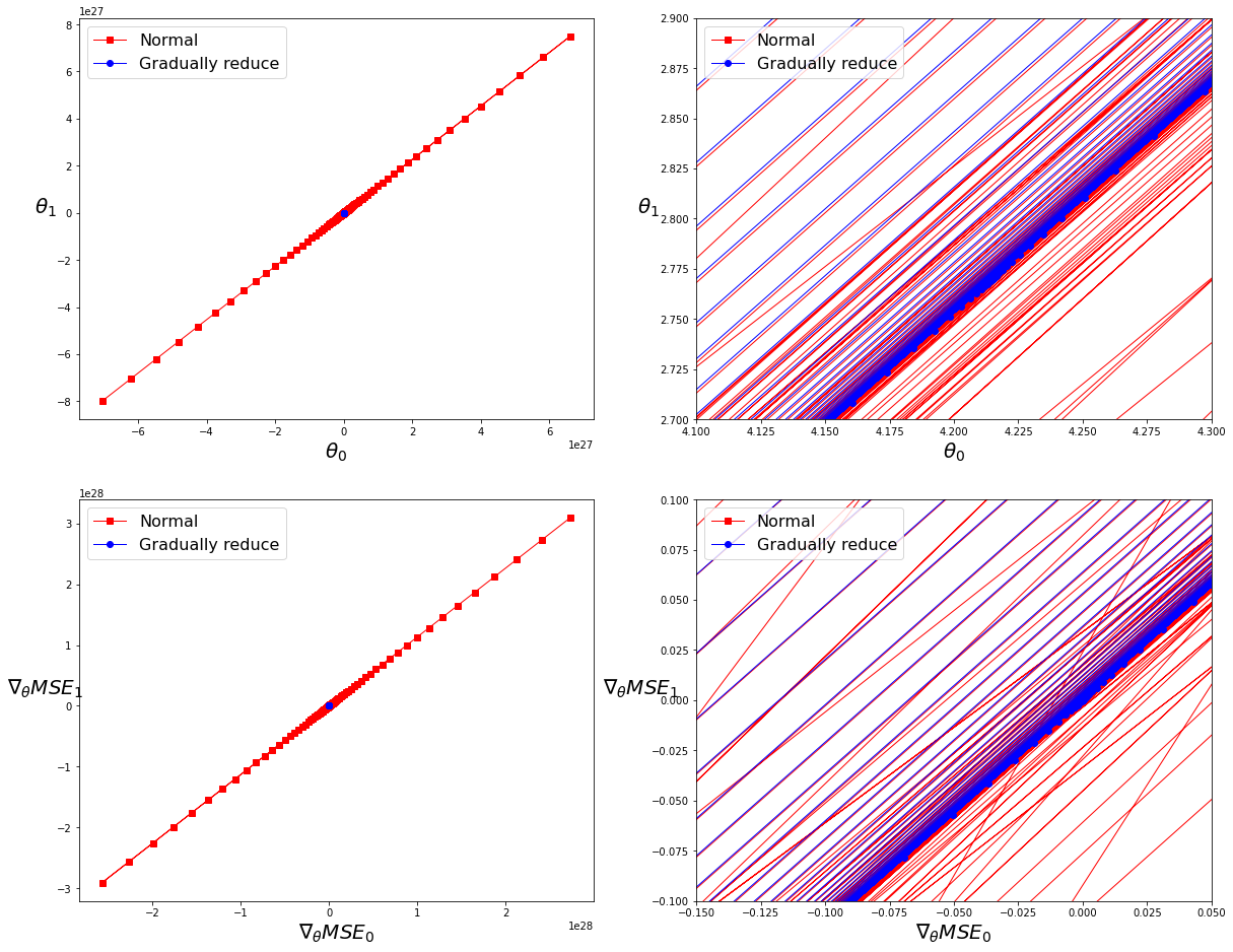
theta_bgd_3[-1], theta_bgd_4[-1]
(array([[-7.05138935e+27],
        [-7.98621001e+27]]),
 array([[4.21509616],
        [2.77011339]]))
3、多项式回归
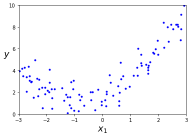
首先,让我们基于一个简单的二次方程式(添加一些噪音)生成一些非线性数据:
np.random.seed(42)
m = 100
X = 6 * np.random.rand(m, 1) - 3
y = 0.5 * X**2 + X + 2 + np.random.randn(m, 1)
from sklearn.preprocessing import PolynomialFeatures
# PolynomialFeatures转换训练数据,将每个特征的平方添加为新特征
poly_features = PolynomialFeatures(degree=2, include_bias=False)
X_poly = poly_features.fit_transform(X)
plt.plot(X, y, "b.")
plt.xlabel("$x_1$", fontsize=18)
plt.ylabel("$y$", rotation=0, fontsize=18)
plt.axis([-3, 3, 0, 10])

plt.show()
X[0], X[0] ** 2, X_poly[0]
(array([-0.75275929]), array([0.56664654]), array([-0.75275929, 0.56664654]))
lin_reg = LinearRegression()
lin_reg.fit(X_poly, y)
lin_reg.intercept_, lin_reg.coef_
(array([1.78134581]), array([[0.93366893, 0.56456263]]))
X_new=np.linspace(-3, 3, 100).reshape(100, 1)
X_new_poly = poly_features.transform(X_new)
y_new = lin_reg.predict(X_new_poly)
plt.plot(X, y, "b.")
plt.plot(X_new, y_new, "r-", linewidth=2, label="Predictions")
plt.xlabel("$x_1$", fontsize=18)
plt.ylabel("$y$", rotation=0, fontsize=18)
plt.legend(loc="upper left", fontsize=14)
plt.axis([-3, 3, 0, 10])

plt.show()
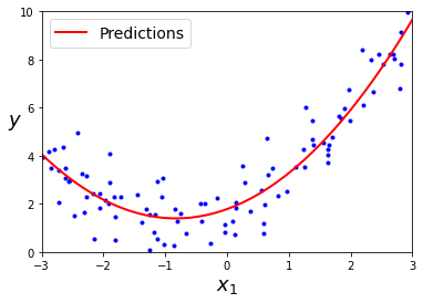
- 预测结果: y = 0.56 x 2 + 0.93 x + 1.78 y = 0.56x^2 + 0.93x + 1.78 y=0.56x2+0.93x+1.78
- 实际结果: y = 0.50 x 2 + 1.00 x + 2.00 + 高 斯 噪 音 y = 0.50x^2 + 1.00x + 2.00 + 高斯噪音 y=0.50x2+1.00x+2.00+高斯噪音
当存在多个特征时,例如,有两个特征a和b,degree=3时,PolynomialFeatures不仅会添加特征
a
2
a^2
a2、
a
3
a^3
a3、
b
2
b^2
b2、
b
3
b^3
b3 还会添加组合
a
b
ab
ab、
a
2
b
a^2b
a2b、
a
b
2
ab^2
ab2 。(即
(
n
+
d
)
!
d
!
n
!
\frac{(n+d)!}{d!n!}
d!n!(n+d)! 个特征组,小心特征数量组合的数量爆炸💥)
4、学习曲线
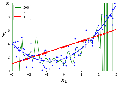
4.1、方法一:泛化性能指标
- 如果模型在训练数据上表现
良好,但是根据交叉验证的泛化指标较差,则模型过拟合。 - 如果两者表现
均不理想,则模型欠拟合。
from sklearn.preprocessing import StandardScaler
from sklearn.pipeline import Pipeline

for style, width, degree in (("g-", 1, 300), ("b--", 2, 2), ("r-+", 2, 1)):
    polybig_features = PolynomialFeatures(degree=degree, include_bias=False)
    std_scaler = StandardScaler()
    lin_reg = LinearRegression()
    polynomial_regression = Pipeline([
            ("poly_features", polybig_features),  # 添加新特征
            ("std_scaler", std_scaler),           # 归一化处理数据
            ("lin_reg", lin_reg),                 # 线性学习
        ])
    polynomial_regression.fit(X, y)
    y_newbig = polynomial_regression.predict(X_new)
    plt.plot(X_new, y_newbig, style, label=str(degree), linewidth=width)

plt.plot(X, y, "b.", linewidth=3)  # 绘制原始数据散点图
plt.legend(loc="upper left")
plt.xlabel("$x_1$", fontsize=18)
plt.ylabel("$y$", rotation=0, fontsize=18)
plt.axis([-3, 3, 0, 10])

plt.show()
4.2、方法二:绘制学习曲线
这个曲线绘制的是模型在训练集和验证集上关于训练集大小(或训练迭代)的性能函数。要生成这个曲线,只需要在不同大小的训练子集上多次训练模型即可。
from sklearn.metrics import mean_squared_error
from sklearn.model_selection import train_test_split


def plot_learning_curves(model, X, y):
    X_train, X_val, y_train, y_val = train_test_split(X, y, test_size=0.2, random_state=10)
    train_errors, val_errors = [], []
    for m in range(1, len(X_train)):
        model.fit(X_train[:m], y_train[:m])
        y_train_predict = model.predict(X_train[:m])
        y_val_predict = model.predict(X_val)
        train_errors.append(mean_squared_error(y_train[:m], y_train_predict))
        val_errors.append(mean_squared_error(y_val, y_val_predict))

    plt.plot(np.sqrt(train_errors), "r-+", linewidth=2, label="train")
    plt.plot(np.sqrt(val_errors), "b-", linewidth=3, label="val")
    plt.legend(loc="upper right", fontsize=14)
    plt.xlabel("Training set size", fontsize=14)
    plt.ylabel("RMSE", fontsize=14)
4.2.1、普通线性回归模型的学习曲线(欠拟合)
lin_reg = LinearRegression()
plot_learning_curves(lin_reg, X, y)
plt.axis([0, 80, 0, 3])

plt.show()
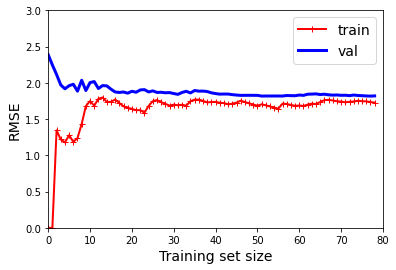
解释一下上图:这是一种欠拟合的模型值
红线:
- 首先,当只有一两个实例时,模型可以很好地拟合它们,这就是曲线从0开始的原因。
- 之后,随着新实例的加入,模型就不可能完美的拟合训练数据,因为数据有噪声。又因为它根本不是线性的。
- 因此,训练数据的误差会一直上升,直到达到平稳状态,此时在训练集中添加新实例并不会是平均误差变好或变坏。
蓝线:
- 首先,当只有一两个实例训练模型时,无法正确的泛化,这就是验证误差最初很大的原因。
- 然后,随着模型训练的实例增加,它开始学习,因此验证错误逐渐降低。
- 但是,直线不能很好地对数据进行建模,因此误差最终达到一个平稳状态,非常接近另一条曲线。
4.2.2、10阶多项式模型的学习曲线(过拟合)
from sklearn.pipeline import Pipeline

polynomial_regression = Pipeline([
    ("poly_features", PolynomialFeatures(degree=10, include_bias=False)),
    ("lin_reg", LinearRegression()),
])

plot_learning_curves(polynomial_regression, X, y)
plt.axis([0, 80, 0, 3])

plt.show()
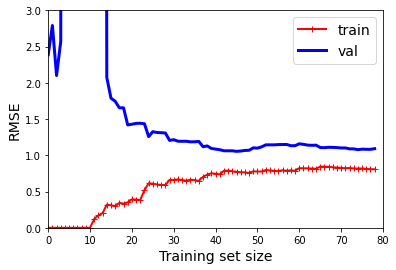
和上一个的区别:
- 与线性回归模型相比,训练数据上的误差要低得多。
- 曲线之间存在
明显间隙。这意味着该模型在训练数据上的性能要比在验证数据上的性能好得多,这是过拟合模型的标志。 - 但是,如果使用
更大的训练集,则两条曲线会继续接近。
改善过拟合模型的一种方法是:向其提供更多的训练数据,直到验证误差到达训练误差为止。
5、正则化线性模拟
正则化(即约束模型)是一个减少过拟合的好方法:模型拥有的自由度越小,则过拟合数据的难度就越大。正则化多项式模型的一种简单方法是减少多项式的次数。
对于线性模型,正则化通常是通过约束模型的权重来实现的。
5.1、岭回归(Tikhonov正则化)
岭回归是线性回归的正则化版本:将等于
α
∑
i
=
0
n
θ
i
2
\alpha\sum_{i=0}^n\theta^2_i
α∑i=0nθi2 的正则化项添加到成本函数。这迫使学习算法不仅拟合数据,而且还使模型权重尽可能小。注意,仅在训练期间将正则化项添加到成本函数中。训练完模型后,你要使用非正则化的性能度量来评估模型的性能。
超参数
α
\alpha
α 控制要对模型进行正则化的程度。如果
α
=
0
\alpha = 0
α=0 ,则岭回归仅是线性回归。如果
α
\alpha
α 非常大,则所有权重最终都非常接近于零,结果是一条经过数据均值的平线。
公式:岭回归成本函数
- J ( θ ) = M S E ( θ ) + α 1 2 ∑ i = 1 n θ i 2 J(\theta) = MSE(\theta) + \alpha\frac{1}{2}\sum\limits_{i=1}^n\theta^2_i J(θ)=MSE(θ)+α21i=1∑nθi2
这里需要注意的是:
- 偏置项 θ 0 \theta_0 θ0 没有进行正则化(总和从 i = 1 i = 1 i=1 开始,而不是 0)。
- 如果我们将 w ⃗ \vec{w} w 定义为特征权重的向量( θ 1 \theta_1 θ1至 θ n \theta_n θn),则正则项等于 1 2 ( ∥ w ⃗ ∥ 2 ) 2 \frac{1}{2}(\|\vec{w}\|_{2})^2 21(∥w∥2)2,其中 ∥ w ⃗ ∥ 2 \|\vec{w}\|_{2} ∥w∥2 表示权重向量的 ι 2 范 数 \iota_2范数 ι2范数。
- 对于梯度下降,只需要将 α w ⃗ \alpha\vec{w} αw 添加到 MSE 梯度向量。
在执行岭回归之前
缩放数据(如使用StandardScaler)很重要,因为它对输入特征的缩放敏感。大多数正则化模型都需要如此。
公式:闭式解的岭回归
- θ ^ = ( X T X + α A ) − 1 X T y \hat{\theta} = (X^TX + \alpha{A})^{-1}X^Ty θ^=(XTX+αA)−1XTy
说明:
- A A A:是一个 ( n + 1 ) × ( n + 1 ) (n+1)×(n+1) (n+1)×(n+1) 单位矩阵。
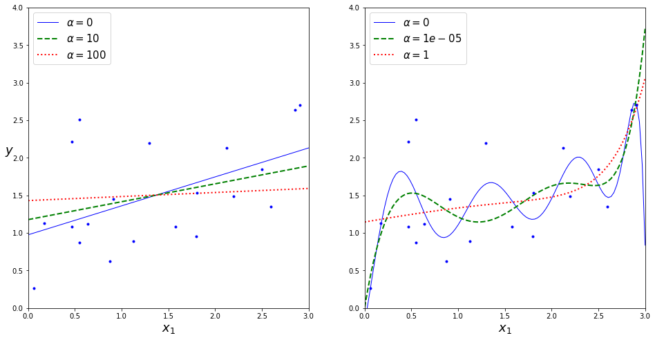
def plot_model(model_class, polynomial, alphas, **model_kargs):
    for alpha, style in zip(alphas, ("b-", "g--", "r:")):
        model = model_class(alpha, **model_kargs) if alpha > 0 else LinearRegression()
        if polynomial:
            model = Pipeline([
                ("poly_features", PolynomialFeatures(degree=10, include_bias=False)),
                ("std_scaler", StandardScaler()),
                ("regul_reg", model),
            ])
        model.fit(X, y)
        y_new_regul = model.predict(X_new)
        lw = 2 if alpha > 0 else 1
        plt.plot(X_new, y_new_regul, style, linewidth=lw,label=r"$\alpha = {}$".format(alpha))
    plt.plot(X, y, "b.", linewidth=3)
    plt.legend(loc="upper left", fontsize=15)
    plt.xlabel("$x_1$", fontsize=18)
    plt.axis([0, 3, 0, 4])
np.random.seed(42)
m = 20
X = 3 * np.random.rand(m, 1)
y = 1 + 0.5 * X + np.random.randn(m, 1) / 1.5
X_new = np.linspace(0, 3, 100).reshape(100, 1)
from sklearn.linear_model import Ridge

plt.figure(figsize=(16, 8))

# 普通线性模型,数据未作处理
plt.subplot(121)
plot_model(Ridge, polynomial=False, alphas=(0, 10, 100), random_state=42)
plt.ylabel("$y$", rotation=0, fontsize=18)

# 多项式模型,数据做了处理。这里的 alphas 范围之所以在 0~1,是因为超过 1,与 1 的曲线相差不大。
plt.subplot(122)
plot_model(Ridge, polynomial=True, alphas=(0, 10**-5, 1), random_state=42)

plt.show()
5.1.1、Scikit-Learn:Ridge
Scikit-Learn 和闭式解(上面公式的一种变体)来执行岭回归的方法:
from sklearn.linear_model import Ridge
ridge_reg = Ridge(alpha=1, solver="cholesky", random_state=42)
ridge_reg.fit(X, y)
ridge_reg.predict([[1.5]])
array([[1.55071465]])
ridge_reg = Ridge(alpha=1, solver="sag", random_state=42)
ridge_reg.fit(X, y)
ridge_reg.predict([[1.5]])
array([[1.5507201]])
- 参数名:solver
- 类型: {‘auto’, ‘svd’, ‘cholesky’, ‘lsqr’, ‘sparse_cg’, ‘sag’, ‘saga’}
- 说明:计算例程中使用的求解程序
| 名称 | 说明 |
|---|---|
| auto | 根据数据类型自动选择求解器 |
| svd | 利用X的奇异值分解来计算脊系数。对于奇异矩阵比“cholesky”更稳定。 |
| cholesky | 使用标准scipy.linalg.solve去得到一个闭合解 |
| sparse_cg | 使用在scipy.sparse.linalg.cg中发现的共轭梯度求解器。作为一种迭代算法,这个求解器比“cholesky”更适合于大规模数据(可以设置tol和max_iter)。 |
| lsqr | 使用专用正规化最小二乘的常规scipy.sparse.linalg.lsqr。它是最快的,但可能不能用旧的scipy版本。它还使用了一个迭代过程。 |
| sag | saga使用随机平均梯度下降改进的,没有偏差的版本,名字为SAGA。这两种方法都使用可迭代的过程,当n_samples和n_feature都很大时,它们通常比其他解决程序更快。 请注意,“sag”和“saga”快速收敛只在具有大致相同规模的特性上得到保证。您可以通过sklearn.preprocessing对数据进行预处理。 |
5.1.2、随机梯度下降法:
超参数penalty设置的是使用正则项的类型。设为l2表示希望SGD在成本函数中添加一个正则项,等于权重向量的
ι
2
范
数
\iota_2范数
ι2范数 的平方的一般,即岭回归。
from sklearn.linear_model import LinearRegression, SGDRegressor

sgd_reg = SGDRegressor(penalty="l2", max_iter=1000, tol=1e-3, random_state=42)
sgd_reg.fit(X, y.ravel())
sgd_reg.predict([[1.5]])
array([1.47012588])
5.2、Lasso 回归
线性回归的另一种正则化叫做最小绝对收缩和选择算子回归(简称 Lasso),与岭回归一样,它也是向成本函数添加一个正则项,但是它增加的是权重向量的
ι
1
范
数
\iota_1范数
ι1范数,而不是
ι
2
范
数
\iota_2范数
ι2范数 的平方的一半:
公式:Lasso 回归成本函数
- J ( θ ) = M S E ( θ ) + α ∑ i = 1 n ∣ θ i ∣ J(\theta) = MSE(\theta) + \alpha\sum\limits_{i=1}^n|\theta_i| J(θ)=MSE(θ)+αi=1∑n∣θi∣
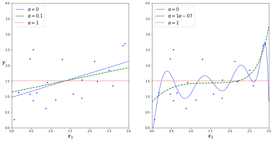
Lasso 回归的一个重要特点是它倾向于完全消除掉最不重要特征的权重(也就是将它们设置为零)。
例如:
- 下图 α = 1 0 − 7 \alpha = 10^{-7} α=10−7 这绿色虚线,看起来像是二次的,快要接近于线性:因为所有高阶多项式的特征权重都等于零。
- 换句话说,Lasso 回归会自动执行特征选择并输出一个稀疏模型(即只有很少的特征有非零权重)。
Lasso回归的特色就是在建立
广义线型模型的时候,这里广义线型模型包含一维连续因变量、多维连续因变量、非负次数因变量、二元离散因变量、多元离散因变,除此之外,无论因变量是连续的还是离散的,Lasso都能处理,总的来说,Lasso对于数据的要求是极其低的,所以应用程度较广;除此之外,Lasso还能够对变量进行筛选和对模型的复杂程度进行降低。这里的变量筛选是指不把所有的变量都放入模型中进行拟合,而是有选择的把变量放入模型从而得到更好的性能参数。 复杂度调整是指通过一系列参数控制模型的复杂度,从而避免过度拟合(Overfitting)。 对于线性模型来说,复杂度与模型的变量数有直接关系,变量数越多,模型复杂度就越高。 更多的变量在拟合时往往可以给出一个看似更好的模型,但是同时也面临过度拟合的危险。
公式:Lasso 回归子梯度向量
- g ( θ , J ) = ∇ θ M S E ( θ ) + α ( sin ( θ 1 ) sin ( θ 2 ) ⋮ sin ( θ n ) ) 其 中 s i g n ( θ i ) = { − 1 如 果 θ i < 0 0 如 果 θ i = 0 + 1 如 果 θ i > 0 g(\theta, J) = \nabla_{\theta} MSE(\theta) + \alpha\begin{pmatrix} \sin \left(\theta_{1}\right) \\ \sin \left(\theta_{2}\right) \\ \vdots \\ \sin \left(\theta_{n}\right) \end{pmatrix}\ \ 其中sign(\theta_i) = \begin{cases} -1\ 如果 \theta_i < 0\\ 0\ \ \ \ 如果 \theta_i = 0\\ +1\ 如果 \theta_i > 0\\ \end{cases} g(θ,J)=∇θMSE(θ)+α⎝⎜⎜⎜⎛sin(θ1)sin(θ2)⋮sin(θn)⎠⎟⎟⎟⎞ 其中sign(θi)=⎩⎪⎨⎪⎧−1 如果θi<00 如果θi=0+1 如果θi>0
5.2.1、Scikit-Learn:Lasso
from sklearn.linear_model import Lasso
lasso_reg = Lasso(alpha=0.1, random_state=42)
lasso_reg.fit(X, y)
lasso_reg.predict([[1.5]])
array([1.53788174])
5.2.2、随机梯度下降法:
超参数penalty设置的是使用正则项的类型。设为l1表示希望SGD在成本函数中添加一个正则项,等于权重向量的
ι
1
范
数
\iota_1范数
ι1范数 的平方的一般,即Lasso回归。
sgd_reg = SGDRegressor(penalty="l1", random_state=42)
sgd_reg.fit(X, y.ravel())
sgd_reg.predict([[1.5]])
array([1.47011206])
from sklearn.linear_model import Lasso

plt.figure(figsize=(16, 8))

# 普通线性模型,数据未作处理
plt.subplot(121)
plot_model(Lasso, polynomial=False, alphas=(0, 0.1, 1), random_state=42)
plt.ylabel("$y$", rotation=0, fontsize=18)

# 多项式模型,数据做了处理。这里的 alphas 范围之所以在 0~1,是因为超过 1,曲线接近直线。
plt.subplot(122)
plot_model(Lasso, polynomial=True, alphas=(0, 10**-7, 1), random_state=42)

plt.show()
/Users/XXXX/site-packages/sklearn/linear_model/_coordinate_descent.py:532: ConvergenceWarning: Objective did not converge. You might want to increase the number of iterations. Duality gap: 2.802867703827432, tolerance: 0.0009294783355207351
  positive)
5.3、Lasso VS 岭正则化
%matplotlib inline
import matplotlib.pyplot as plt
import numpy as np
t1a, t1b, t2a, t2b = -1, 3, -1.5, 1.5

t1s = np.linspace(t1a, t1b, 500)
t2s = np.linspace(t2a, t2b, 500)
t1, t2 = np.meshgrid(t1s, t2s)
T = np.c_[t1.ravel(), t2.ravel()]
Xr = np.array([[1, 1], [1, -1], [1, 0.5]])
yr = 2 * Xr[:, :1] + 0.5 * Xr[:, 1:]

J = (1/len(Xr) * np.sum((T.dot(Xr.T) - yr.T)**2, axis=1)).reshape(t1.shape)

N1 = np.linalg.norm(T, ord=1, axis=1).reshape(t1.shape)
N2 = np.linalg.norm(T, ord=2, axis=1).reshape(t1.shape)

t_min_idx = np.unravel_index(np.argmin(J), J.shape)
t1_min, t2_min = t1[t_min_idx], t2[t_min_idx]

t_init = np.array([[0.25], [-1]])
def bgd_path(theta, X, y, l1, l2, core = 1, eta = 0.05, n_iterations = 200):
    path = [theta]
    for iteration in range(n_iterations):
        gradients = core * 2/len(X) * X.T.dot(X.dot(theta) - y) + l1 * np.sign(theta) + l2 * theta
        theta = theta - eta * gradients
        path.append(theta)
    return np.array(path)

fig, axes = plt.subplots(2, 2, sharex=True, sharey=True, figsize=(20.2, 16))
for i, N, l1, l2, title in ((0, N1, 2., 0, "Lasso"), (1, N2, 0,  2., "Ridge")):
    JR = J + l1 * N1 + l2 * 0.5 * N2**2

    tr_min_idx = np.unravel_index(np.argmin(JR), JR.shape)
    t1r_min, t2r_min = t1[tr_min_idx], t2[tr_min_idx]

    levelsJ=(np.exp(np.linspace(0, 1, 20)) - 1) * (np.max(J) - np.min(J)) + np.min(J)
    levelsJR=(np.exp(np.linspace(0, 1, 20)) - 1) * (np.max(JR) - np.min(JR)) + np.min(JR)
    levelsN=np.linspace(0, np.max(N), 10)

    path_J = bgd_path(t_init, Xr, yr, l1=0, l2=0)
    path_JR = bgd_path(t_init, Xr, yr, l1, l2)
    path_N = bgd_path(np.array([[2.0], [0.5]]), Xr, yr, np.sign(l1)/3, np.sign(l2), core=0)

    ax = axes[i, 0]
    ax.grid(True)
    ax.axhline(y=0, color='k')
    ax.axvline(x=0, color='k')
    ax.contourf(t1, t2, N / 2., levels=levelsN)
    ax.plot(path_N[:, 0], path_N[:, 1], "y--")
    ax.plot(0, 0, "ys")
    ax.plot(t1_min, t2_min, "ys")
    ax.set_title(r"$\ell_{}$ penalty".format(i + 1), fontsize=16)
    ax.axis([t1a, t1b, t2a, t2b])
    if i == 1:
        ax.set_xlabel(r"$\theta_1$", fontsize=16)
    ax.set_ylabel(r"$\theta_2$", fontsize=16, rotation=0)

    ax = axes[i, 1]
    ax.grid(True)
    ax.axhline(y=0, color='k')
    ax.axvline(x=0, color='k')
    ax.contourf(t1, t2, JR, levels=levelsJR, alpha=0.9)
    ax.plot(path_JR[:, 0], path_JR[:, 1], "w-o")
    ax.plot(path_N[:, 0], path_N[:, 1], "y--")
    ax.plot(0, 0, "ys")
    ax.plot(t1_min, t2_min, "ys")
    ax.plot(t1r_min, t2r_min, "rs")
    ax.set_title(title, fontsize=16)
    ax.axis([t1a, t1b, t2a, t2b])
    if i == 1:
        ax.set_xlabel(r"$\theta_1$", fontsize=16)

plt.show()
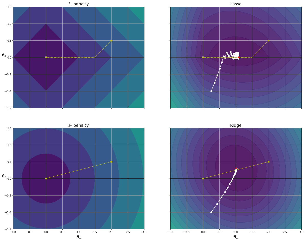
上面左侧图片,背景代表梯度降低的趋势,而黄线则是实际运动轨迹。
-
θ
1
\theta_1
θ1 和
θ
2
\theta_2
θ2 是同密度下降,所有左上角先
45°的方向线性下降, θ 2 \theta_2 θ2优先到达 0,减少了一个维度的数据(优先去除不重要的变量),从而降低了模型的复杂度。 -
θ
1
\theta_1
θ1 和
θ
2
\theta_2
θ2 是同密度下降,所有左下角直接
向原点的方向直线下降,这也意味着,无法真正较少数据维度,只能趋近于零。
上面右侧图片,背景代表成本函数的趋势,而白圈代表梯度下降优化某些模型参数的路径。
- 但是右上角(白圈代表梯度下降优化某些模型参数的路径)先快速到达全局最优解附近,然后不断调整并最终在全局最优值
附近反弹。 - 右下角与Lasso有两个主要不同:
2.1. 首先,随着参数接近全局最优值,梯度会变小,因此,梯度下降自然减慢,有助于收敛,不会有明显的反弹。
2.2. 其次,当你增加 α \alpha α 时,最佳参数(红色方形小点)越来越接近原点,但是它们从未被消除(也就是没有减少数据维度,只是无线接近于0)。
5.4、弹性网络
弹性网络是介于岭回归和Lasso回归之间的中间地带。正则项是岭和Lasso正则项的简单混合,你可以控制混合比
r
r
r。
- 当
r
=
0
r = 0
r=0时,弹性网络等效于
岭回归; - 当
r
=
1
r = 1
r=1时,弹性网络等效于
Lasso回归;
公式:弹性网络成本函数
- J ( θ ) = M S E ( θ ) + r α ∑ i = 1 n ∣ θ i ∣ + 1 − r 2 α ∑ i = 1 n θ i 2 J(\theta) = MSE(\theta) + r\alpha\sum\limits_{i=1}^n|\theta_i| + \frac{1 - r}{2}\alpha\sum\limits_{i=1}^n\theta^2_i J(θ)=MSE(θ)+rαi=1∑n∣θi∣+21−rαi=1∑nθi2
那么什么时候应该使用普通的线性回归(即不进行任何正则化)、岭、Lasso或弹性网络呢?通常来讲,有正则化–哪怕很小,总比没有更可取一些,所以大多数情况下,你应该避免使用纯线性回归。
岭回归是个不错的默认选择;- 但是如果你觉得实际用到的特征只有少数几个,那就应该更倾向于
Lasso回归或是弹性网络,因为它们会将无用特征的权重将为零; - 一般而言,
弹性网络优于Lasso回归,因为当特征数量超过训练实例数量,又或是几个特征强相关时,Lasso回归的表现可能非常不稳定。
下面使用弹性网络(Scikit-Learn 的 ElasticNet)的示例:
- l1_ratio:混合比 r r r
from sklearn.linear_model import ElasticNet

elastic_net = ElasticNet(alpha=0.1, l1_ratio=0.5, random_state=42)
elastic_net.fit(X, y)
elastic_net.predict([[1.5]])
array([1.54333232])
5.5、提前停止
对于梯度下降这一类迭代学习的算法,还有一个与众不同的正则方法,就是在验证误差达到最小值时停止训练,该方法叫做提前停止法。
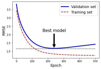
下面展示一个用批量梯度下降训练的复杂模型(高阶多项式回归模型)。经过一轮一轮的训练(即同一组训练集,重复训练多次),算法不断地学习,训练集上的预测误差(RMSE)自然不断下降,同样其在验证集上的预测误差也随之下降。但是,一段时间之后,验证误差停止下降反而开始回升。这说明模型开始过拟合训练数据。通过早起停止法,一旦验证误差达到最小值就立刻停止训练。这是一个非常简单而有效的正则化技巧,所以被称之为“美丽的免费午餐”。
例: y = X + 0.5 X 2 + 2 + 噪 音 ( − 3 < X < 3 ) y = X + 0.5X^2 + 2 + 噪音 (-3 < X < 3) y=X+0.5X2+2+噪音(−3<X<3)
np.random.seed(42)
m = 100
X = 6 * np.random.rand(m, 1) - 3
y = 2 + X + 0.5 * X**2 + np.random.randn(m, 1)

X_train, X_val, y_train, y_val = train_test_split(X[:50], y[:50].ravel(), test_size=0.5, random_state=10)
from copy import deepcopy
# 数据处理:
poly_scaler = Pipeline([
        # 添加新特征(包含无用特征)
        ("poly_features", PolynomialFeatures(degree=90, include_bias=False)),
        # 标准化,特征缩放
        ("std_scaler", StandardScaler())
    ])
# 数据转化
X_train_poly_scaled = poly_scaler.fit_transform(X_train)
X_val_poly_scaled = poly_scaler.transform(X_val)
# 高阶多项式回归模型
sgd_reg = SGDRegressor(max_iter=1, tol=-np.infty, warm_start=True,
                       penalty=None, learning_rate="constant", eta0=0.0005, random_state=42)

minimum_val_error = float("inf")  # 当前最小值,默认值:正无穷
best_epoch = None                 # 最佳时期(即 验证误差达到最小值)
best_model = None                 # 最佳模型
rmse_list = []
for epoch in range(1000):
    sgd_reg.fit(X_train_poly_scaled, y_train)             # 连续训练模型,而不是从头开始
    y_val_predict = sgd_reg.predict(X_val_poly_scaled)    # 预测
    val_error = mean_squared_error(y_val, y_val_predict)  # 验证误差
    rmse_list.append(val_error)
    if val_error < minimum_val_error:   # 如果 验证误差 < 当前最小值
        minimum_val_error = val_error   # 记录当前最小值
        best_epoch = epoch              # 记录最佳时期
        best_model = deepcopy(sgd_reg)  # 记录最佳模型
# 绘制 验证误差曲线
plt.plot(range(1000), rmse_list)
plt.axhline(y=rmse_list[best_epoch],ls=":",c="red")
plt.axvline(x=best_epoch,ls=":",c="red")
plt.xlabel("Training Number", fontsize=14)
plt.ylabel("RMSE", fontsize=14)
plt.show()
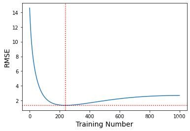
best_epoch, best_model
(239,
 SGDRegressor(eta0=0.0005, learning_rate='constant', max_iter=1, penalty=None,
              random_state=42, tol=-inf, warm_start=True))
sgd_reg = SGDRegressor(max_iter=1, tol=-np.infty, warm_start=True,
                       penalty=None, learning_rate="constant", eta0=0.0005, random_state=42)

n_epochs = 500
train_errors, val_errors = [], []
for epoch in range(n_epochs):
    sgd_reg.fit(X_train_poly_scaled, y_train)
    y_train_predict = sgd_reg.predict(X_train_poly_scaled)
    y_val_predict = sgd_reg.predict(X_val_poly_scaled)
    train_errors.append(mean_squared_error(y_train, y_train_predict))
    val_errors.append(mean_squared_error(y_val, y_val_predict))

best_epoch = np.argmin(val_errors)
best_val_rmse = np.sqrt(val_errors[best_epoch])

plt.annotate('Best model',
             xy=(best_epoch, best_val_rmse),
             xytext=(best_epoch, best_val_rmse + 1),
             ha="center",
             arrowprops=dict(facecolor='black', shrink=0.05),
             fontsize=16,
            )

best_val_rmse -= 0.03  # just to make the graph look better
plt.plot([0, n_epochs], [best_val_rmse, best_val_rmse], "k:", linewidth=2)
plt.plot(np.sqrt(val_errors), "b-", linewidth=3, label="Validation set")
plt.plot(np.sqrt(train_errors), "r--", linewidth=2, label="Training set")
plt.legend(loc="upper right", fontsize=14)
plt.xlabel("Epoch", fontsize=14)
plt.ylabel("RMSE", fontsize=14)

plt.show()
6、逻辑回归
一些回归算法也可用于分类(反之亦然)。逻辑回归(也称 Logit 回归)被广泛用于估算一个实例属于某个特定类别的概率(比如,一封电子邮件,属于垃圾邮件的概率)。如果预估概率超过 50%,则模型预测该实例属于该类(称为 正类,标记为 1),反之,则预测不是(称为 负类,标记为 0)。这样它就成了一个二元分类器。
6.1、估计概率
与线性归回模型一样,逻辑回归模型也是计算输入特征的加权和(加上偏置项),但是不同于线性回归模型直接输出结果,它输出的是结果的数值逻辑
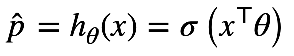
公式:逻辑回归模型的估计概率(向量化形式)
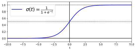
逻辑记为
σ
(
⋅
)
\sigma(·)
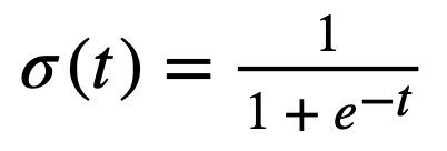
σ(⋅),是一个 sigmoid 函数(即 S 型函数),输出一个介于 0 和 1 之间的数字。
其公式如下:
公式:逻辑函数
t = np.linspace(-10, 10, 100)
sig = 1 / (1 + np.exp(-t))
plt.figure(figsize=(9, 3))
plt.plot([-10, 10], [0, 0], "k-")
plt.plot([-10, 10], [0.5, 0.5], "k:")
plt.plot([-10, 10], [1, 1], "k:")
plt.plot([0, 0], [-1.1, 1.1], "k-")
plt.plot(t, sig, "b-", linewidth=2, label=r"$\sigma(t) = \frac{1}{1 + e^{-t}}$")
plt.xlabel("t")
plt.legend(loc="upper left", fontsize=20)
plt.axis([-10, 10, -0.1, 1.1])

plt.show()
一旦逻辑回归模型估算出实例X属于正类的概率
p
^
=
h
θ
(
x
)
\hat{p}=h_{\theta}(x)
p^=hθ(x),就可以轻松做出预测
y
^
\hat{y}
y^:
公式:逻辑回归模型预测
- y ^ = { 0 , 如 果 p ^ < 0.5 1 , 如 果 p ^ > 0.5 \hat{y} = \begin{cases} 0, \ \ \ \ \ 如果 \hat{p} < 0.5\\ 1, \ \ \ \ \ 如果 \hat{p} > 0.5\\ \end{cases} y^={0, 如果p^<0.51, 如果p^>0.5
6.2、训练和成本函数
训练的目的就是设置参数向量
θ
\theta
θ,使模型对正类实例做出高概率估算(
y
=
1
y = 1
y=1),对负类实例做出低概率估算(
y
=
0
y = 0
y=0)。
下面公式所示为单个训练实例X的成本函数,正说明这一点。
公式:单个训练实例的成本函数
-
c ( θ ) = { − l o g ( p ^ ) , 如 果 y = 1 − l o g ( 1 − p ^ ) , 如 果 y = 0 c(\theta) = \begin{cases} -log(\hat{p})\ \ \ \ \ \ \ \ \ , 如果 y = 1\\ -log(1-\hat{p})\ \ , 如果 y = 0\\ \end{cases} c(θ)={−log(p^) ,如果y=1−log(1−p^) ,如果y=0
-
当 t 接近于 0 时, − l o g ( t ) -log(t) −log(t) 会变得非常大,所以如果模型估算一个正类实例的概率接近于 0,成本将会变得非常高。同理,估算出一个负类实例的概率接近于 1,成本也会变得非常高。
-
当 t 接近于 1 时, − l o g ( t ) -log(t) −log(t) 会接近于 0,所以如果模型估算一个正类实例的概率接近于 1,成本将则都接近于 0。同理,估算出一个负类实例的概率接近于 0,成本也接近于 0。
-
所以,尽可能的让 t 接近于 1。
整个训练集的成本函数时所有训练实例的平均成本。可以用一个称为对数损失对的单一表达式来表示。
公式:逻辑回归成本函数(对数损失)
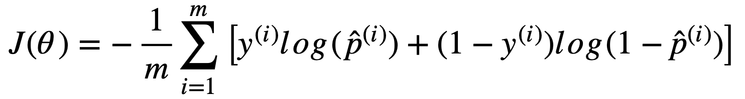
但是坏事消息是,整个函数没有已知的闭式方程(不存在一个标准方程的等价方程)来计算出最小化成本函数的
θ
\theta
θ 值。而好消息是这是个凸函数,所以可以通过梯度下降(或者其他任意优化算法)保证能找出全局最小值(只要学习率不太高,你又能长时间等待)。
这里给出了成本函数关于第
j
j
j 个模型参数
θ
j
\theta_j
θj 的偏导数方程。
公式:逻辑成本函数偏导数
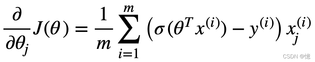
与2.1的成本函数非常相似。
6.3、决策边界
这里我们用鸢尾植物数据集来说明逻辑回归。这是一个非常知名的数据集,共有150朵鸢尾花,分别来自三个不同品种(山鸢尾。变色鸢尾和维吉尼亚鸢尾),数据里包含花的萼片以及花瓣的长度和宽度。
from sklearn import datasets
iris = datasets.load_iris()
list(iris.keys())
['data',
 'target',
 'frame',
 'target_names',
 'DESCR',
 'feature_names',
 'filename']
print(iris.DESCR) # 说明
.. _iris_dataset:

Iris plants dataset
--------------------

**Data Set Characteristics:**

    :Number of Instances: 150 (50 in each of three classes)
    :Number of Attributes: 4 numeric, predictive attributes and the class
    :Attribute Information:
        - sepal length in cm
        - sepal width in cm
        - petal length in cm
        - petal width in cm
        - class:
                - Iris-Setosa
                - Iris-Versicolour
                - Iris-Virginica

    :Summary Statistics:

    ============== ==== ==== ======= ===== ====================
                    Min  Max   Mean    SD   Class Correlation
    ============== ==== ==== ======= ===== ====================
    sepal length:   4.3  7.9   5.84   0.83    0.7826
    sepal width:    2.0  4.4   3.05   0.43   -0.4194
    petal length:   1.0  6.9   3.76   1.76    0.9490  (high!)
    petal width:    0.1  2.5   1.20   0.76    0.9565  (high!)
    ============== ==== ==== ======= ===== ====================

    :Missing Attribute Values: None
    :Class Distribution: 33.3% for each of 3 classes.
    :Creator: R.A. Fisher
    :Donor: Michael Marshall (MARSHALL%PLU@io.arc.nasa.gov)
    :Date: July, 1988

The famous Iris database, first used by Sir R.A. Fisher. The dataset is taken
from Fisher's paper. Note that it's the same as in R, but not as in the UCI
Machine Learning Repository, which has two wrong data points.

This is perhaps the best known database to be found in the
pattern recognition literature.  Fisher's paper is a classic in the field and
is referenced frequently to this day.  (See Duda & Hart, for example.)  The
data set contains 3 classes of 50 instances each, where each class refers to a
type of iris plant.  One class is linearly separable from the other 2; the
latter are NOT linearly separable from each other.

.. topic:: References

   - Fisher, R.A. "The use of multiple measurements in taxonomic problems"
     Annual Eugenics, 7, Part II, 179-188 (1936); also in "Contributions to
     Mathematical Statistics" (John Wiley, NY, 1950).
   - Duda, R.O., & Hart, P.E. (1973) Pattern Classification and Scene Analysis.
     (Q327.D83) John Wiley & Sons.  ISBN 0-471-22361-1.  See page 218.
   - Dasarathy, B.V. (1980) "Nosing Around the Neighborhood: A New System
     Structure and Classification Rule for Recognition in Partially Exposed
     Environments".  IEEE Transactions on Pattern Analysis and Machine
     Intelligence, Vol. PAMI-2, No. 1, 67-71.
   - Gates, G.W. (1972) "The Reduced Nearest Neighbor Rule".  IEEE Transactions
     on Information Theory, May 1972, 431-433.
   - See also: 1988 MLC Proceedings, 54-64.  Cheeseman et al"s AUTOCLASS II
     conceptual clustering system finds 3 classes in the data.
   - Many, many more ...
6.3.1、一个维度(花瓣宽度)
X = iris["data"][:, 3:]  # 花瓣宽度
y = (iris["target"] == 2).astype(np.int)  # 1 表示 维吉尼亚鸢尾,否则为 0
训练一个逻辑回归模型:
from sklearn.linear_model import LogisticRegression
log_reg = LogisticRegression(solver="lbfgs", random_state=42)
log_reg.fit(X, y)
LogisticRegression(random_state=42)
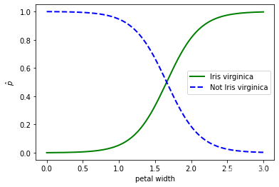
我们来看看花瓣宽度在 0~3cm 之间的鸢尾花,模型估算出来的概率:
X_new = np.linspace(0, 3, 1000).reshape(-1, 1)
y_proba = log_reg.predict_proba(X_new)

plt.plot(X_new, y_proba[:, 1], "g-", linewidth=2, label="Iris virginica")
plt.plot(X_new, y_proba[:, 0], "b--", linewidth=2, label="Not Iris virginica")
plt.xlabel('petal width')
plt.ylabel('$\hat{p}$')
plt.legend()
<matplotlib.legend.Legend at 0x7fd3c8d98310>
X_new = np.linspace(0, 3, 1000).reshape(-1, 1)
y_proba = log_reg.predict_proba(X_new)
decision_boundary = X_new[y_proba[:, 1] >= 0.5][0]

plt.figure(figsize=(8, 3))
plt.plot(X[y==0], y[y==0], "bs")
plt.plot(X[y==1], y[y==1], "g^")
plt.plot([decision_boundary, decision_boundary], [-1, 2], "k:", linewidth=2)
plt.plot(X_new, y_proba[:, 1], "g-", linewidth=2, label="Iris virginica")
plt.plot(X_new, y_proba[:, 0], "b--", linewidth=2, label="Not Iris virginica")
plt.text(decision_boundary+0.02, 0.15, "Decision  boundary", fontsize=14, color="k", ha="center")
plt.arrow(decision_boundary, 0.08, -0.3, 0, head_width=0.05, head_length=0.1, fc='b', ec='b')
plt.arrow(decision_boundary, 0.92, 0.3, 0, head_width=0.05, head_length=0.1, fc='g', ec='g')
plt.xlabel("Petal width (cm)", fontsize=14)
plt.ylabel("Probability", fontsize=14)
plt.legend(loc="center left", fontsize=14)
plt.axis([0, 3, -0.02, 1.02])

plt.show()
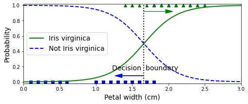
上图是《估计的概率和决策边界》
- 维吉尼亚鸢尾(三角形所示)的花瓣宽度范围为 1.4~2.5cm
- 而其他两种鸢尾花(正方形所示)花瓣通常较窄,花瓣宽度范围 0.1~1.8cm
- 注意,这里有部分重叠
- 所以,在 1.6cm 处存在一个决策边界,这里“是”与“不是”的可能性都是 50%。
log_reg.predict([[1.7], [1.5]])
array([1, 0])
6.3.2、两个维度(花瓣宽度,花瓣长度)
- 控制
Scikit-LearnLogisticRegression模型的正则化强度的超参数不是alpha,而是反值C。C值越高,对模型的正则化越少。
from sklearn.linear_model import LogisticRegression

X = iris["data"][:, (2, 3)]  # 花瓣长度, 花瓣宽度
y = (iris["target"] == 2).astype(np.int)

log_reg = LogisticRegression(solver="lbfgs", C=10**10, random_state=42)
log_reg.fit(X, y)

x0, x1 = np.meshgrid(
        np.linspace(2.9, 7, 500).reshape(-1, 1),
        np.linspace(0.8, 2.7, 200).reshape(-1, 1),
    )
X_new = np.c_[x0.ravel(), x1.ravel()]

y_proba = log_reg.predict_proba(X_new)

plt.figure(figsize=(10, 4))
plt.plot(X[y==0, 0], X[y==0, 1], "bs")
plt.plot(X[y==1, 0], X[y==1, 1], "g^")

zz = y_proba[:, 1].reshape(x0.shape)
contour = plt.contour(x0, x1, zz, cmap=plt.cm.brg)


left_right = np.array([2.9, 7])
boundary = -(log_reg.coef_[0][0] * left_right + log_reg.intercept_[0]) / log_reg.coef_[0][1]

plt.clabel(contour, inline=1, fontsize=12)
plt.plot(left_right, boundary, "k--", linewidth=3)
plt.text(3.5, 1.5, "Not Iris virginica", fontsize=14, color="b", ha="center")
plt.text(6.5, 2.3, "Iris virginica", fontsize=14, color="g", ha="center")
plt.xlabel("Petal length", fontsize=14)
plt.ylabel("Petal width", fontsize=14)
plt.axis([2.9, 7, 0.8, 2.7])

plt.show()
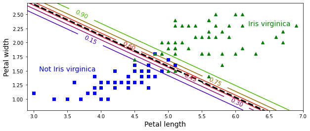
还是相同的数据集,但是这次显示了两个特征:花瓣宽度和花瓣长度。
- 经过训练,这个逻辑回归分类器就可以基于这两个特征来预测新花朵是否属于维吉尼亚鸢尾。
- 虚线表示:模型估算概率为 50% 的点,即模型的决策边界。注意,这里是一个线性边界。
- 每条平行线都分别代表一个模型输出的特定概率,从左下的 15% 到右上的 90%。
- 根据这个模型,右上线之上的所有花朵都有超过 90% 的概率属于 维吉尼亚鸢尾。
与其他线性模型一样,逻辑回归模型可以用
l
1
l_1
l1 或
l
2
l_2
l2 惩罚函数来正则化。Scikit-Learn默认添加的是
l
2
l_2
l2 函数。
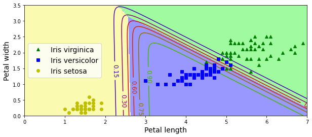
6.4、Softmax 回归(多元逻辑回归)
逻辑回归模型经过推广,可以直接支持多个类型,而不需要训练并组合多个二元分类器。这就是 Softmax回归,或者叫做多元逻辑回归。
原理很简单:给定一个实例
x
x
x,Softmax回归模型首选计算出每个类
k
k
k 的分数
S
k
(
x
)
S_k(x)
Sk(x),然后对这些分数应用Softmax函数(也叫归一化指数),估算出每个类的概率。你应该很熟悉计算
S
k
(
x
)
S_k(x)
Sk(x) 分数公式。因为它看起来就跟线性回归预测方程一样。
公式:类 k 的 Softmax 分数
- S k ( x ) = x T θ ( k ) S_k(x) = x^T\theta^{(k)} Sk(x)=xTθ(k)
请注意,每个类都有自己的特征参数向量 θ ( k ) \theta^{(k)} θ(k)。所有这些向量通常都作为行存储在数据矩阵 Θ \Theta Θ 中。
一旦为实例
x
x
x 计算了每个类的分数,就可以通过 Softmax函数 来估计实例属于类
k
k
k 的概率
p
k
^
\hat{p_k}
pk^。该函数计算每个分数的指数,然后对其进行归一化(除以所有指数总和)。分数通常称为对数或对数奇数(尽管他们实际上是未归一化的对数奇数).
公式:Softmax 函数
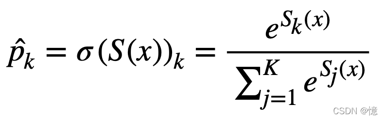
在此等式中:
- K:是类数
- s ( x ) s(x) s(x):是一个向量,其中包含实例 x x x 的每个类的分数。
- σ ( s ( x ) ) k \sigma(s(x))_k σ(s(x))k:是实例 x x x 属于类 k k k 的估计概率,给定该实例每个类的分数。
就像逻辑回归分类器一样,Softmax回归分类器预测具有最高估计概率的类(简单来说就是得分最高的类),如下面公式:
公式:Softmax 回归分类预测
- y ^ = a r g m a x σ ( S ( x ) ) k = a r g m a x S k ( x ) = a r g m a x ( ( θ ( k ) ) T x \hat{y} = argmax \sigma(S(x))_k = argmax S_k(x) = argmax((\theta^{(k)})^Tx y^=argmaxσ(S(x))k=argmaxSk(x)=argmax((θ(k))Tx
argmax运算符返回使函数最大化的变量值。在此等式中,他返回使估计概率
σ
(
S
(
x
)
)
k
\sigma(S(x))_k
σ(S(x))k 最大化的
k
k
k 值。
Softmax回归分类器一次只能预测一个类(即便是多类,而不是多输出),因此它只能与互斥的类(例如不同的植物)一起使用。无法使用它在一张照片中识别多个人。
X = iris["data"][:, (2, 3)]  # 花瓣长度, 花瓣宽度
y = iris["target"]

# multi_class:训练模式;solver:求解器;C:正则化强度,越高,正则化越少
softmax_reg = LogisticRegression(multi_class="multinomial",solver="lbfgs", C=10, random_state=42)
softmax_reg.fit(X, y)
LogisticRegression(C=10, multi_class='multinomial', random_state=42)
x0, x1 = np.meshgrid(
        np.linspace(0, 8, 500).reshape(-1, 1),
        np.linspace(0, 3.5, 200).reshape(-1, 1),
    )
X_new = np.c_[x0.ravel(), x1.ravel()]


y_proba = softmax_reg.predict_proba(X_new)
y_predict = softmax_reg.predict(X_new)

zz1 = y_proba[:, 1].reshape(x0.shape)
zz = y_predict.reshape(x0.shape)

plt.figure(figsize=(10, 4))
plt.plot(X[y==2, 0], X[y==2, 1], "g^", label="Iris virginica")
plt.plot(X[y==1, 0], X[y==1, 1], "bs", label="Iris versicolor")
plt.plot(X[y==0, 0], X[y==0, 1], "yo", label="Iris setosa")

from matplotlib.colors import ListedColormap
custom_cmap = ListedColormap(['#fafab0','#9898ff','#a0faa0'])

plt.contourf(x0, x1, zz, cmap=custom_cmap)
contour = plt.contour(x0, x1, zz1, cmap=plt.cm.brg)
plt.clabel(contour, inline=1, fontsize=12)
plt.xlabel("Petal length", fontsize=14)
plt.ylabel("Petal width", fontsize=14)
plt.legend(loc="center left", fontsize=14)
plt.axis([0, 7, 0, 3.5])

plt.show()


 15万+
15万+


 被折叠的 条评论
为什么被折叠?
被折叠的 条评论
为什么被折叠?
 到【灌水乐园】发言


