【Tensorflow】tf.nn.depthwise_conv2d如何实现深度卷积?+深度可分离卷积详解

本文链接：https://blog.csdn.net/weixin_43135178/article/details/116202785

本文介绍了深度可分离卷积，包括逐通道卷积和逐点卷积的操作原理，参数对比，以及在MobileNet等轻量网络中的应用。通过代码实例展示了如何使用TensorFlow实现depthwise_conv2d，并对比了常规卷积的参数节省。

摘要生成于 C知道，由 DeepSeek-R1 满血版支持，前往体验 >

一些轻量级的网络，如mobilenet中，会有深度可分离卷积depthwise separable convolution，由depthwise(DW)和pointwise(PW)两个部分结合起来，用来提取特征feature map，相比常规的卷积操作，其参数数量和运算成本比较低

常规卷积操作

对于一张5×5像素、三通道（shape为5×5×3），经过3×3卷积核的卷积层（假设输出通道数为4，则卷积核shape为3×3×3×4，最终输出4个Feature Map，
如果有same padding则输出尺寸与输入层相同（5×5×4），如果没有则为尺寸变为3×3×4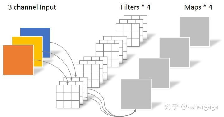

卷积层共4个Filter，每个Filter包含了3个Kernel，每个Kernel的大小为3×3。因此卷积层的参数数量可以用如下公式来计算：N_std = 4 × 3 × 3 × 3 = 108

深度可分离卷积 = 逐通道卷积+逐点卷积

1.逐通道卷积

Depthwise Convolution的一个卷积核负责一个通道，一个通道只被一个卷积核卷积

一张5×5像素、三通道彩色输入图片（shape为5×5×3），Depthwise Convolution首先经过第一次卷积运算，DW完全是在二维平面内进行。卷积核的数量与上一层的通道数相同（通道和卷积核一一对应）。所以一个三通道的图像经过运算后生成了3个Feature map(如果有same padding则尺寸与输入层相同为5×5)，如下图所示。

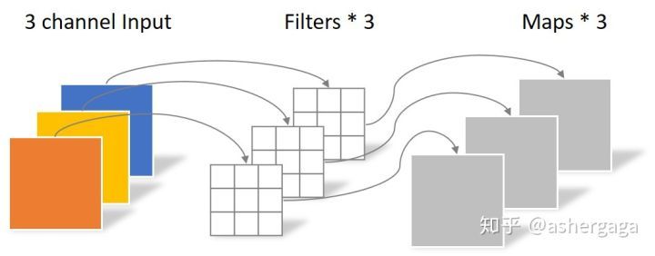
其中一个Filter只包含一个大小为3×3的Kernel，卷积部分的参数个数计算如下：N_depthwise = 3 × 3 × 3 = 27

Depthwise Convolution完成后的Feature map数量与输入层的通道数相同，无法扩展Feature map。而且这种运算对输入层的每个通道独立进行卷积运算，没有有效的利用不同通道在相同空间位置上的feature信息。因此需要Pointwise Convolution来将这些Feature map进行组合生成新的Feature map

2.逐点卷积

Pointwise Convolution的运算与常规卷积运算非常相似，它的卷积核的尺寸为 1×1×M，M为上一层的通道数。所以这里的卷积运算会将上一步的map在深度方向上进行加权组合，生成新的Feature map。有几个卷积核就有几个输出Feature map

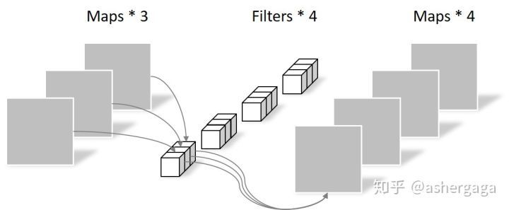
由于采用的是1×1卷积的方式，此步中卷积涉及到的参数个数可以计算为：N_pointwise = 1 × 1 × 3 × 4 = 12

经过Pointwise Convolution之后，同样输出了4张Feature map，与常规卷积的输出维度相同

参数对比

回顾一下，常规卷积的参数个数为：
N_std = 4 × 3 × 3 × 3 = 108

Separable Convolution的参数由两部分相加得到：
N_depthwise = 3 × 3 × 3 = 27
N_pointwise = 1 × 1 × 3 × 4 = 12
N_separable = N_depthwise + N_pointwise = 39

相同的输入，同样是得到4张Feature map，Separable Convolution的参数个数是常规卷积的约1/3。因此，在参数量相同的前提下，采用Separable Convolution的神经网络层数可以做的更深。

介绍

depthwise_conv2d来源于深度可分离卷积:

tf.nn.depthwise_conv2d(input,filter,strides,padding,rate=None,name=None,data_format=None)

除去name参数用以指定该操作的name，data_format指定数据格式，与方法有关的一共五个参数：

input：
指需要做卷积的输入图像，要求是一个4维Tensor，具有[batch, height, width, in_channels]这样的shape，具体含义是[训练时一个batch的图片数量, 图片高度, 图片宽度, 图像通道数]

filter：
相当于CNN中的卷积核，要求是一个4维Tensor，具有[filter_height, filter_width, in_channels, channel_multiplier]这样的shape，具体含义是[卷积核的高度，卷积核的宽度，输入通道数，输出卷积乘子]，同理这里第三维in_channels，就是参数value的第四维

strides：
卷积的滑动步长。

padding：
string类型的量，只能是”SAME”,”VALID”其中之一，这个值决定了不同边缘填充方式。

rate：
这个参数的详细解释见【Tensorflow】tf.nn.atrous_conv2d如何实现空洞卷积？

结果返回一个Tensor，shape为[batch, out_height, out_width, in_channels * channel_multiplier]，注意这里输出通道变成了 in_channels * channel_multiplier

实验

为了形象的展示depthwise_conv2d，我们必须要建立自定义的输入图像和卷积核

img1 = tf.constant(value=[[[[1],[2],[3],[4]],[[1],[2],[3],[4]],[[1],[2],[3],[4]],[[1],[2],[3],[4]]]],dtype=tf.float32)
img2 = tf.constant(value=[[[[1],[1],[1],[1]],[[1],[1],[1],[1]],[[1],[1],[1],[1]],[[1],[1],[1],[1]]]],dtype=tf.float32)
img = tf.concat(values=[img1,img2],axis=3)

filter1 = tf.constant(value=0, shape=[3,3,1,1],dtype=tf.float32)
filter2 = tf.constant(value=1, shape=[3,3,1,1],dtype=tf.float32)
filter3 = tf.constant(value=2, shape=[3,3,1,1],dtype=tf.float32)
filter4 = tf.constant(value=3, shape=[3,3,1,1],dtype=tf.float32)
filter_out1 = tf.concat(values=[filter1,filter2],axis=2)
filter_out2 = tf.concat(values=[filter3,filter4],axis=2)
filter = tf.concat(values=[filter_out1,filter_out2],axis=3)

建立好了img和filter，就可以做卷积了

out_img = tf.nn.conv2d(input=img, filter=filter, strides=[1,1,1,1], padding='VALID')

好了，用一张图来详细展示这个过程
这里写图片描述

这里写图片描述

这是普通的卷积过程，我们再来看深度卷积。

out_img = tf.nn.depthwise_conv2d(input=img, filter=filter, strides=[1,1,1,1], rate=[1,1], padding='VALID')

这里写图片描述

现在我们可以形象的解释一下depthwise_conv2d卷积了。看普通的卷积，我们对卷积核每一个out_channel的两个通道分别和输入的两个通道做卷积相加，得到feature map的一个channel，而depthwise_conv2d卷积，我们对每一个对应的in_channel，分别卷积生成两个out_channel，所以获得的feature map的通道数量可以用in_channel* channel_multiplier来表达，这个channel_multiplier，就可以理解为卷积核的第四维。

代码清单

import tensorflow as tf


img1 = tf.constant(value=[[[[1],[2],[3],[4]],[[1],[2],[3],[4]],[[1],[2],[3],[4]],[[1],[2],[3],[4]]]],dtype=tf.float32)
img2 = tf.constant(value=[[[[1],[1],[1],[1]],[[1],[1],[1],[1]],[[1],[1],[1],[1]],[[1],[1],[1],[1]]]],dtype=tf.float32)
img = tf.concat(values=[img1,img2],axis=3)
filter1 = tf.constant(value=0, shape=[3,3,1,1],dtype=tf.float32)
filter2 = tf.constant(value=1, shape=[3,3,1,1],dtype=tf.float32)
filter3 = tf.constant(value=2, shape=[3,3,1,1],dtype=tf.float32)
filter4 = tf.constant(value=3, shape=[3,3,1,1],dtype=tf.float32)
filter_out1 = tf.concat(values=[filter1,filter2],axis=2)
filter_out2 = tf.concat(values=[filter3,filter4],axis=2)
filter = tf.concat(values=[filter_out1,filter_out2],axis=3)

out_img = tf.nn.depthwise_conv2d(input=img, filter=filter, strides=[1,1,1,1], rate=[1,1], padding='VALID')

输出：

rate=1, VALID mode result:
[[[[  0.  36.   9.  27.]
   [  0.  54.   9.  27.]]

  [[  0.  36.   9.  27.]
   [  0.  54.   9.  27.]]]]

原文连接：https://blog.csdn.net/mao_xiao_feng/article/details/78003476

https://zhuanlan.zhihu.com/p/92134485