


1.分类问题
1.1 准备MNIST数据集
- MNIST数据集:是一个入门级的计算机视觉数据集,它包含各种手写数字图片。
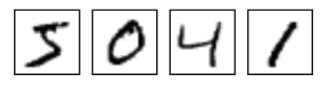
它也包含每一张图片对应的标签,告诉我们这个是数字几。比如,上面这四张图片的标签分别是5,0,4,1。 - MNIST数据集下载:官网地址
- 导入方式:
import input_data
mnist = input_data.read_data_sets("文件路径",one_hot=true)
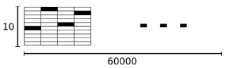
- one_hot编码:一个one-hot向量除了某一位的数字是1以外其余各维度数字都是0。比如,标签0将表示成([1,0,0,0,0,0,0,0,0,0,0])。
1.2 预测MNIST手写数据集
import tensorflow as tf
import matplotlib.pyplot as plt
from tensorflow.examples.tutorials.mnist import input_data
mnist = input_data.read_data_sets('MNIST_data/', one_hot=True)
def simple_layer(inputs, input_size, output_size):
"""
封装一层神经网络
:param inputs: 数据
:param input_size: 行数
:param output_size: 列数
:return: 无
"""
w = tf.Variable(tf.truncated_normal([input_size,output_size]))
# w = tf.Variable(tf.random_normal([input_size,output_size]))
b = tf.Variable(tf.zeros([output_size])+0.1)
return tf.matmul(inputs,w) + b
def draw_graph(data_array,x_label,y_label,name,order):
"""
绘制loss图像
:param data_array: 数据
:param x_label: x轴名称
:param y_label: y轴名称
:param name: 图表名称
:return: 无
"""
plt.figure(order)
plt.plot(data_array)
plt.xlabel(x_label)
plt.ylabel(y_label)
plt.title("lr={0} tr={1} bs={2}".format(learning_rate,train_epochs,batch_size))
plt.savefig(name,dpi=200)
tf.reset_default_graph() #重置图
#参数设置
learning_rate = 0.01 #学习率
train_epochs = 500 #训练轮数
batch_size = 100 #一批数据的大小为100
display_step = 50 #展示的步长
loss_record = [] #储存loss
accuracy_record = [] #存储accuracy
x = tf.placeholder(tf.float32, [None, 784]) #mnist 维度28*28 = 784
y = tf.placeholder(tf.float32, [None, 10]) #表示0-9个数字的
#预测层
pred = tf.nn.softmax(simple_layer(x,784,10))
#反向传播,将生成的pred与y进行一次交叉熵运算最小化误差cost
loss = tf.reduce_mean(-tf.reduce_sum(y * tf.log(pred), reduction_indices=1)) #reduce_sum是按列求和
#梯度下降优化器
optimizer = tf.train.GradientDescentOptimizer(learning_rate=learning_rate).minimize(loss)
correct_prediction = tf.equal(tf.argmax(pred, 1), tf.argmax(y, 1))
accuracy = tf.reduce_mean(tf.cast(correct_prediction, tf.float32))
init = tf.global_variables_initializer()
saver = tf.train.Saver() #获取保存对象
model_path = "mn/model.cpkt" #设置保存模型的位置
#启动session,训练模型
with tf.Session() as sess:
sess.run(init) #初始化全部的值
#启动循环开始训练
for epoch in range(train_epochs):
train_loss_epoch = 0
train_accuracy_epoch = 0
#将图片分组
total_batch = int(mnist.train.num_examples/batch_size)
#遍历全部数据集
for i in range(total_batch):
#获取一个批次的数据
batch_xs, batch_ys = mnist.train.next_batch(batch_size)
#启动optimizer优化器
sess.run(optimizer,feed_dict={x:batch_xs,y:batch_ys})
# pred_s = sess.run(pred,feed_dict={x:batch_xs,y:batch_ys})
# print(pred_s)
train_loss = sess.run(loss, feed_dict={x:batch_xs, y:batch_ys})
train_correct = sess.run(accuracy, feed_dict={x:batch_xs, y:batch_ys})
#计算一次epochs的误差与准确率
train_loss_epoch += train_loss / total_batch
train_accuracy_epoch += train_correct / total_batch
#显示训练中的详细信息,50步展示一次
if (epoch+1) % display_step == 0:
print("Epoch:", '%04d'%(epoch+1), " lost=", '{:.9f}'.format(train_loss_epoch)," accuracy=", "{:.4f}".format(train_accuracy_epoch))
loss_record.append(train_loss_epoch)
accuracy_record.append(train_accuracy_epoch)
print("Training finished!")
#测试model
correct_prediction = tf.equal(tf.argmax(pred, 1), tf.argmax(y, 1))
#计算准确率
accuracy = tf.reduce_mean(tf.cast(correct_prediction, tf.float32))
print("测试集准确率:", accuracy.eval({x:mnist.test.images, y:mnist.test.labels}))
#存储模型
save_path = saver.save(sess, model_path)
print("Model saved in file:%s"%save_path)
#绘制图表
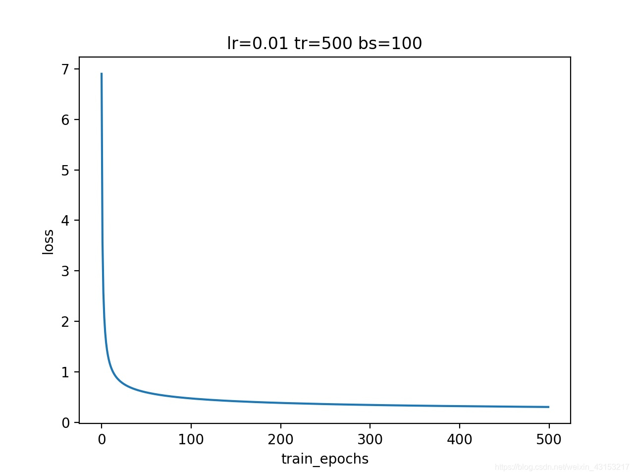
draw_graph(loss_record,"train_epochs","loss","loss_graph.jpg",1)
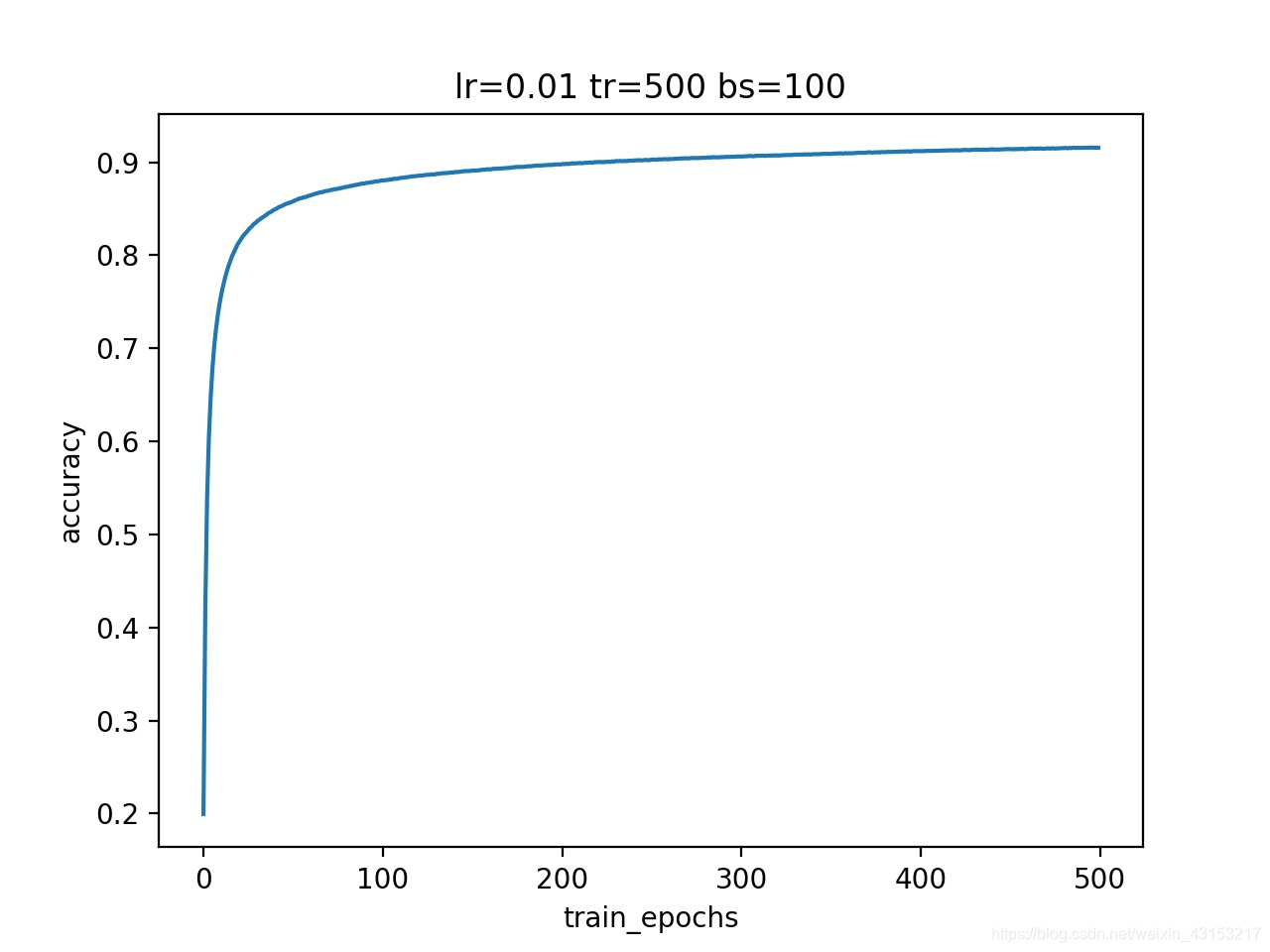
draw_graph(accuracy_record,"train_epochs","accuracy","accuracy_graph.jpg",2)
print("Graph saved")
Output:
Epoch: 0050 lost= 0.599896277 accuracy= 0.8571
Epoch: 0100 lost= 0.477679570 accuracy= 0.8802
Epoch: 0150 lost= 0.421992446 accuracy= 0.8907
Epoch: 0200 lost= 0.388164593 accuracy= 0.8975
Epoch: 0250 lost= 0.364874119 accuracy= 0.9023
Epoch: 0300 lost= 0.347681733 accuracy= 0.9061
Epoch: 0350 lost= 0.334310911 accuracy= 0.9089
Epoch: 0400 lost= 0.323556781 accuracy= 0.9119
Epoch: 0450 lost= 0.314724997 accuracy= 0.9140
Epoch: 0500 lost= 0.307318334 accuracy= 0.9155
Training finished!
测试集准确率: 0.9117
Model saved in file:mn/model.cpkt
Graph saved
loss
accuracy
2.欠拟合与过拟合
- 图示
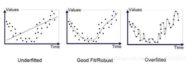
2.1 什么是欠拟合?
- 概念:如图一Underfitted,是模型简单或者说语料集偏少、特征太多,在训练集上的准确率不高,同时在测试集上的准确率也不高,这样如何训练都无法训练出有意义的参数,模型也得不到较好的效果。
2.2 如何避免欠拟合?
-
1,添加其他特征项,模型出现欠拟合的时候是因为特征项不够导致的,可以添加其他特征项来很好地解决。
例如,“组合”、“泛化”、“相关性”三类特征是特征添加的重要手段, 无论在什么场景,都可以照葫芦画瓢,总会得到意想不到的效果。 除上面的特征之外,“上下文特征”、“平台特征”等等,都可以作为特征添加的首选项。 -
2,添加多项式特征,例如将线性模型通过添加二次项或者三次项使模型泛化能力更强。
-
3,减少正则化参数,正则化的目的是用来防止过拟合的,当模型出现了欠拟合,则需要减少正则化参数。
2.3 什么是过拟合?
- 概念:如图三Overfitted,具体表现在:深度学习的模型在提供的训练集上表现的效果非常好,但是在未经过训练集观察的测试集上,模型的效果很差,即输出的泛化能力很弱。
2.4 如何避免过拟合?
- 1,获取和使用更多的数据集
- 对于解决过拟合的办法就是给与足够多的数据集,让模型在更多的数据上进行“观察”和拟合,从而不断修正自己。然而不可能收集无限多的数据集,因此一个常用的方法就是调整已有数据,添加大量的噪音,或者对图形进行锐化,旋转,明暗度调整等优化。
- 2,采用合适的模型
- 目前来说,基于不同的情况和分类要求,对使用的模型也不同。过于简单或者过于复杂都会导致过拟合问题。
- 3,使用dropout
- dropout是一个非常有用和常用的方法。dropout层指的是模型在训练过程中每次按50%的几率关闭或忽略某些层的节点。使得模型在使用同样的数据进行训练时相当于从不同的模型中随机选择一个进行训练。
- 4,权重衰减
- 权重衰减(Weight-decay)又被称为正则化。具体的做法是将权重加入到损失函数中。
- Loss = loss + reg(wi)
- 在实际中使用L1正则和L2正则:
- L1 = λ/n * Σ|wi| 所有的权重w值求和,乘以λ/n
- L2 = λ/2n * Σ(wi)^2 所有的权重w的平方求和,乘以λ/2n
- 5,Early Stopping
- Early stoppin是参数微调的一种,即在每个循环结束一次以后(这里的循环可能是full data batch,也可能是mini batch size),计算模型的准确率(accuracy)。当准确率不在增加时就停止训练。
- 6,使用Batch Normalization。参见7.Batch Normalization
3.CNN(卷积神经网络)
3.1 什么是CNN?
- 概念:卷积神经网络(Convolutional Neural Networks, CNN)是一类包含卷积计算且具有深度结构的前馈神经网络(Feedforward Neural Networks),是深度学习(deep learning)的代表算法之一。
- 卷积函数原型:tf.nn.conv2d(inputs,filter,strides,padding,use_cudnn_on_gpu=None,name=None)
- inputs:需要做卷积处理的输入图像,要求是一个张量(tensor),具有[batch,in_height,in_width,in_channels],具体含义[训练时一批图片的数量,图像高度,图像宽度,图像通道数]。
- filter:是CNN中的卷积核,要求是一个tensor,具有[filter_height,filter_width,in_channels,out_channels],具体含义[卷积核的高度,卷积核的宽度,输入图像的通道数,输出图像的通道数]。
- strides:卷积时在每一维的步长,[1,strides1,strides2,1]第一维和第四维默认为1,第三维和第四维分别是平行和竖直滑行的步进长度。
- padding:string类型的量,只能是"SAME",“VALID”,SAME会在卷积计算时,在外围会补齐0,而VALID不会补齐0。
- use_cudnn_on_gpu:bool类型是否使用cudnn加速,默认为true。
- 卷积计算:
- padding="SAME"时,卷积后图像为out_height=in_height/strides1,out_width=out_width/strides2。
- padding="VALID"时,卷积后的图像为out_height=(in_height-filter_hieght+1)/strides1,out_width=(in_width-filter_width+1)/strides2。
- 卷积图解:
- 计算的移动

- 计算的移动
3.2 搭建一个CNN
- 以MNIST数据集为例,添加卷积层
- 示例代码
import tensorflow as tf
import matplotlib.pyplot as plt
from tensorflow.examples.tutorials.mnist import input_data
mnist = input_data.read_data_sets('MNIST_data/', one_hot=True)

def weights(shape):
    return tf.Variable(tf.truncated_normal(shape))

def simple_layer(inputs, input_size, output_size):
    """
    封装一层神经网络
    :param inputs: 数据
    :param input_size: 行数
    :param output_size: 列数
    :return: 无
    """
    w = tf.Variable(tf.truncated_normal([input_size,output_size]))
    # w = tf.Variable(tf.random_normal([input_size,output_size]))
    b = tf.Variable(tf.zeros([output_size])+0.1)
    return tf.matmul(inputs,w) + b

def conv2d_layer(inputs,filter,strides,padding,activation=None):
    output = tf.nn.conv2d(inputs,filter,strides,padding)
    return activation(output)

def max_pooling(inputs,kernel_size,strides,padding):
    return tf.nn.max_pool(inputs,kernel_size,strides,padding)

def draw_graph(data_array,x_label,y_label,name,order):
    """
    绘制loss图像
    :param data_array: 数据
    :param x_label: x轴名称
    :param y_label: y轴名称
    :param name: 图表名称
    :return: 无
    """
    plt.figure(order)
    plt.plot(data_array)
    plt.xlabel(x_label)
    plt.ylabel(y_label)
    plt.title("lr={0} tr={1} bs={2}".format(learning_rate,train_epochs,batch_size))
    plt.savefig(name,dpi=200)

#参数设置
learning_rate = 0.001   #学习率
train_epochs = 500  #训练轮数
batch_size = 50   #一批数据的大小为100
display_step = 1   #展示的步长
loss_record = []   #储存loss
accuracy_record = []   #存储accuracy

x = tf.placeholder(tf.float32, [None, 784])   #mnist 维度28*28 = 784
y = tf.placeholder(tf.float32, [None, 10])    #表示0-9个数字的

x_image = tf.reshape(x,[-1,28,28,1])   #将[None,784]转换为[None,28,28,1]的形状
#卷积层
conv2d_layer1 = conv2d_layer(x_image,weights([5,5,1,16]),[1,1,1,1],"SAME",tf.nn.relu)
conv2d_pooling1 = max_pooling(conv2d_layer1,[1,2,2,1],[1,2,2,1],"SAME")    #[14,14,16]
#卷积层
conv2d_layer2 = conv2d_layer(conv2d_pooling1,weights([5,5,16,32]),[1,1,1,1],"SAME",tf.nn.relu)
conv2d_pooling2 = max_pooling(conv2d_layer2,[1,2,2,1],[1,2,2,1],"SAME")    #[7,7,32]

reshape = tf.reshape(conv2d_pooling2,[-1,7*7*32])   #展平[7*7*32]
#全连接层
pred = tf.nn.softmax(simple_layer(reshape,7*7*32,10))

#反向传播,将生成的pred与y进行一次交叉熵运算最小化误差cost
# loss = tf.reduce_mean(-tf.reduce_sum(y * tf.log(pred), reduction_indices=1))   #reduce_sum是按列求和
loss = tf.reduce_mean(tf.nn.softmax_cross_entropy_with_logits(labels=y,logits=pred))
#梯度下降优化器
optimizer = tf.train.AdamOptimizer(learning_rate=learning_rate).minimize(loss)
correct_prediction = tf.equal(tf.argmax(pred, 1), tf.argmax(y, 1))
accuracy = tf.reduce_mean(tf.cast(correct_prediction, tf.float32))
init = tf.global_variables_initializer()

saver = tf.train.Saver()   #获取保存对象
model_path = "CNN/model.cpkt"     #设置保存模型的位置

#启动session,训练模型
with tf.Session() as sess:
    sess.run(init)    #初始化全部的值

    #启动循环开始训练
    for epoch in range(train_epochs):
        train_loss_epoch = 0
        train_accuracy_epoch = 0

        #将图片分组
        total_batch = int(mnist.train.num_examples/batch_size)

        #遍历全部数据集
        for i in range(total_batch):
            #获取一个批次的数据
            batch_xs, batch_ys = mnist.train.next_batch(batch_size)

            #启动optimizer优化器
            sess.run(optimizer,feed_dict={x:batch_xs,y:batch_ys})
            # pred_s = sess.run(pred,feed_dict={x:batch_xs,y:batch_ys})
            # print(pred_s)
            train_loss = sess.run(loss, feed_dict={x:batch_xs, y:batch_ys})
            train_correct = sess.run(accuracy, feed_dict={x:batch_xs, y:batch_ys})

            #计算一次epochs的误差与准确率
            train_loss_epoch += train_loss / total_batch
            train_accuracy_epoch += train_correct / total_batch

        #显示训练中的详细信息,50步展示一次
        if (epoch+1) % display_step == 0:
            print("Epoch:", '%04d'%(epoch+1), " lost=", '{:.6f}'.format(train_loss_epoch)," accuracy=", "{:.6f}".format(train_accuracy_epoch))
        loss_record.append(train_loss_epoch)
        accuracy_record.append(train_accuracy_epoch)

    print("Training finished!")

    #存储模型
    save_path = saver.save(sess, model_path)
    print("Model saved in file:%s"%save_path)
    #绘制图表
    draw_graph(loss_record,"train_epochs","loss","CNN_loss_graph.jpg",1)
    draw_graph(accuracy_record,"train_epochs","accuracy","CNN_accuracy_graph.jpg",2)
    print("Graph saved")
4.saver 模型的存取
4.1 模型的存储
- 示例代码:
saver = tf.train.Saver()
save_path = "mn/model.cpkt"   #保存位置
saver.save(sess,save_path)  #保存现在的sess
4.2 模型的读取
- 示例代码:
saver = tf.train.Saver()
#读取训练好的模型到当前会话sess
saver.restore(sess,tf.train.latest_checkpoint(".//mn"))  #保存的文件夹
5.Batch Normalization
5.1 理解Batch Normalization
- 一般来说,当模型设计完毕后,更多的是需要对输入的数据进行处理,不同的数据类型以及图片属性都会对模型的训练产生很大的影响。因此需要一种专门的方法去解决因图片不同而产生的差异影响。
- 对于深度学习来说,数据在模型中训练是一个复杂的过程。即使训练模型网络的前面几层发生非常微小的变化,随着梯度下降算法的计算,这个微小的变化在后面几层也会被累积放大下去。
- 当数据输入的属性分布发生改变时,即使是很微小的变化,在传递这个变化的过程时,网络的后端也会产生非常大的变化,从而需要整个模型,整个网络去重新适应和学习这个新的数据分布。如果训练的数据分布一直在发生变化,那么训练模型对最后的预测结果也是在一个比较大的错误率之间浮动。
- Batch_Normalization是一种新近的对数据差异性进行处理的手段,归一化就是将数据的输入值减去其均值然后除以数据的标准差。通过对在“一个范围内”的数据进行规范化处理,使得输出结果的均值为0,方差为1。
- 好处:对数据进行了一定程度上预处理,使得无论是训练数据集还是测试集都在一定范围内进行分布和波动,对数据点中包含的误差进行掩盖化处理,增强模型的泛化能力。
5.2 Batch Normalization的运用
- TensorFlow提供了专门的函数来完成数据的Batch_Normalization的计算。
- batch_normalization(x,mean,variance,offset,scale,variance_epsilon,name)
- x:输入的数据文件。
- mean:批量数据方差。
- variance:批量数据方差。
- offset:待训练的参数。
- scale:待训练的参数。
- variance_eplilon:方差编译系数。
- name:名称。
- 这里主要使用了Batch中的均值以及方差。offset和scale是在模型中需要训练的数据。variance_epsilon是需要设定的一个系数,一般情况下将其设置为0.0001。
- batch_normalization(x,mean,variance,offset,scale,variance_epsilon,name)


 2325
2325


 被折叠的 条评论
为什么被折叠?
被折叠的 条评论
为什么被折叠?
 到【灌水乐园】发言


