


最近博主申请了一个大创项目,做的是计算机视觉方面的(给自己挖了一个天坑),为了补天,只能硬着头皮上了。考虑到numpy这个库在计算机视觉领域是一个很重要的库,于是决定阅读一下numpy的tutorial。鉴于博主英语战五渣,所以,读不通的地方,还请大家自行脑补
以下文字翻译自numpy QuickStart tutorial,原文地址:
https://docs.scipy.org/doc/numpy/user/quickstart.html
同时参考了另一篇关于numpy QuickStart tutorial的博客,
原文地址:
https://blog.csdn.net/shenlongshi/article/details/53812099
(下面开始正文)
先决条件
在你阅读这篇教程之前, 你需要对python有一些了解。如果你想要复习一下之前所学,你可以阅读Python tutorial。
如果你希望运行这个教程中的范例,你的计算机中必须要安装一些软件。请在https://scipy.org/install.html中了解更多。
基本
Numpy的主要对象是异构的多维数组,这个数组通常是一些相同类型的元素的表格(这些元素通常是数组),由一个元组的正整数索引。在NumPy中,维度被叫做坐标轴。
例如,一个3D空间中的一个点的坐[1, 2, 1] 有一个坐标轴,这个坐标轴中有3个元素,所以我们称这个坐标轴的长度为3。在下面的示例中,这个数组有两个坐标轴,。第一个坐标轴长度为2,第二个坐标轴长度为3。
[[ 1., 0., 0.],
 [ 0., 1., 2.]]
Numpy的数组类被称为ndarray 。它也被称为array。需要注意的是,numpy.array和Standard Python Library 提供的类 array.array 不一样,后者只能处理一元数组,且功能更少。下面列出来的是在一个ndarray中较为重要的属性:
ndarray.ndim
一个数组坐标轴(维度)的数量
ndarray.shape
数组的维度。这是一个表示在每个维度数组中数组大小的整数元组。对于一个n行m列的矩阵,它的shape是(n, m)。shape元组的长度是坐标轴的数量,ndim。
ndarray.size
一个数组元素的总数。它等价于shape中各个元素的乘积。
ndarray.dtype
一个形容数组中元素类型的对象。你可以使用python标准类型来创造或声明一个dtype。另外,NumPy也提供其独有的类型。例如numpy.int32,numpy.int16,和numpy.float64。
ndarray.itemsize
一个数组的元素的大小。例如,一个元素类型是float64的数组的itemsize是8(=64/8)。一个元素类型是complex32的数组的itemsize是4(=32/8)。它和ndarray.dtype.itemsize等价。
ndarray.data
一个承装数组真实元素的缓存区。一般地,我们不会调用这个属性,因为我们会使用索引来使用数组中的元素。
一个范例
>>> import numpy as np
>>> a = np.arange(15).reshape(3, 5)
>>> a
array([[ 0,  1,  2,  3,  4],
       [ 5,  6,  7,  8,  9],
       [10, 11, 12, 13, 14]])
>>> a.shape
(3, 5)
>>> a.ndim
2
>>> a.dtype.name
'int64'
>>> a.itemsize
8
>>> a.size
15
>>> type(a)
<type 'numpy.ndarray'>
>>> b = np.array([6, 7, 8])
>>> b
array([6, 7, 8])
>>> type(b)
<type 'numpy.ndarray'>
数组的创建
下面将介绍一些创建数组的方式。
例如,你可以通过调用函数array来使用常规python的列表或元组来创建一个数组。创建出来的数组的元素类型将通过序列元素类型推断。
>>> import numpy as np
>>> a = np.array([2,3,4])
>>> a
array([2, 3, 4])
>>> a.dtype
dtype('int64')
>>> b = np.array([1.2, 3.5, 5.1])
>>> b.dtype
dtype('float64')
一个在调用array时出现的创建错误是填入一些数字参数,而不是提供一个单独的数字列表作为参数。
>>> a = np.array(1,2,3,4)    # WRONG
>>> a = np.array([1,2,3,4])  # RIGHT
array会将一个二重嵌套序列转换成二维数组,将三重嵌套序列转换成三位数组,以此类推。
>>> b = np.array([(1.5,2,3), (4,5,6)])
>>> b
array([[ 1.5,  2. ,  3. ],
       [ 4. ,  5. ,  6. ]])
数组的类型也可以创建的时候单独声明:
>>> c = np.array( [ [1,2], [3,4] ], dtype=complex )
>>> c
array([[ 1.+0.j,  2.+0.j],
      [ 3.+0.j,  4.+0.j]])
有时候,一个数组的元素在最初时并不知道,但是它的规模是知道的。因此,NumPy提供了一些通过最初的占位符来创建数组的函数。这使得创建一个数组所需要的代价最小化。
函数zeros创建一个元素全0的数组,函数ones创建一个元素全为1的数组,函数emtpy创建一个初始元素为根据内存状态产生的随机数。一般地,生成数组的dtype是float64。
>>> np.zeros( (3,4) )
array([[ 0.,  0.,  0.,  0.],
       [ 0.,  0.,  0.,  0.],
       [ 0.,  0.,  0.,  0.]])
>>> np.ones( (2,3,4), dtype=np.int16 )                # dtype can also be specified
array([[[ 1, 1, 1, 1],
        [ 1, 1, 1, 1],
        [ 1, 1, 1, 1]],
       [[ 1, 1, 1, 1],
        [ 1, 1, 1, 1],
        [ 1, 1, 1, 1]]], dtype=int16)
>>> np.empty( (2,3) )                                 # uninitialized, output may vary
array([[  3.73603959e-262,   6.02658058e-154,   6.55490914e-260],
       [  5.30498948e-313,   3.14673309e-307,   1.00000000e+000]])
为了创造一个数字序列 ,NumPy提供一个类似于range的函数,来返回一个数组,而不是列表。
>>> np.arange( 10, 30, 5 )
array([10, 15, 20, 25])
>>> np.arange( 0, 2, 0.3 )                 # it accepts float arguments
array([ 0. ,  0.3,  0.6,  0.9,  1.2,  1.5,  1.8])
当一arange接受了浮点数参数时,因为有限的浮点精度,它一般很难判断出元素的数值。因此,最好是通过函数linspace来接受我们想要元素的参数,就像这样:
>>> from numpy import pi
>>> np.linspace( 0, 2, 9 )                 # 9 numbers from 0 to 2
array([ 0.  ,  0.25,  0.5 ,  0.75,  1.  ,  1.25,  1.5 ,  1.75,  2.  ])
>>> x = np.linspace( 0, 2*pi, 100 )        # useful to evaluate function at lots of points
>>> f = np.sin(x)
参考
array, zeros, zeros_like, ones, ones_like, empty, empty_like, arrange, lispace, numpy.random.rand, numpy.random.randn, fromfunction, fromfile
打印数组
当你打印一个数组时,NumPy将和显示一个嵌套列表一样显示,但是会根据下列规范:
- 最后一个坐标轴从左至右打,
- 倒数第二个坐标轴从上到下打印
- 剩下的坐标轴同样从上到下打印,每个分片之间由一个空行间隔开来
一维数组打印成行,二维数组打印成矩阵,三位数组打印成矩阵列表
>>> a = np.arange(6)                         # 1d array
>>> print(a)
[0 1 2 3 4 5]
>>>
>>> b = np.arange(12).reshape(4,3)           # 2d array
>>> print(b)
[[ 0  1  2]
 [ 3  4  5]
 [ 6  7  8]
 [ 9 10 11]]
>>>
>>> c = np.arange(24).reshape(2,3,4)         # 3d array
>>> print(c)
[[[ 0  1  2  3]
  [ 4  5  6  7]
  [ 8  9 10 11]]
 [[12 13 14 15]
  [16 17 18 19]
  [20 21 22 23]]]
阅读下面(改变数组形状)一节来了解关于reshape的细节
如果一个数组过大以至于无法打印,NumPy将自动地跳数组的中间部分,只打印角落处的内容。
>>> print(np.arange(10000))
[   0    1    2 ..., 9997 9998 9999]
>>>
>>> print(np.arange(10000).reshape(100,100))
[[   0    1    2 ...,   97   98   99]
 [ 100  101  102 ...,  197  198  199]
 [ 200  201  202 ...,  297  298  299]
 ...,
 [9700 9701 9702 ..., 9797 9798 9799]
 [9800 9801 9802 ..., 9897 9898 9899]
 [9900 9901 9902 ..., 9997 9998 9999]]
为了使这个功能失效并且强制NumPy打印整个数组,你可以调用set_printoptions更改输出选项。
>>> np.set_printoptions(threshold=np.nan)
基础操作
数组的数学运算使用逐个元素运算的方案。产生结果时,一个数组被创建然后被填充入结果。
>>> a = np.array( [20,30,40,50] )
>>> b = np.arange( 4 )
>>> b
array([0, 1, 2, 3])
>>> c = a-b
>>> c
array([20, 29, 38, 47])
>>> b**2
array([0, 1, 4, 9])
>>> 10*np.sin(a)
array([ 9.12945251, -9.88031624,  7.4511316 , -2.62374854])
>>> a<35
array([ True, True, False, False])
不同于许多矩阵语言,乘号*在NumPy按照逐个元素相乘的策略。矩阵乘法可以通过@运算符(在python3.5及以上)或者dot函数实现:
>>> A = np.array( [[1,1],
...             [0,1]] )
>>> B = np.array( [[2,0],
...             [3,4]] )
>>> A * B                       # elementwise product
array([[2, 0],
       [0, 4]])
>>> A @ B                       # matrix product
array([[5, 4],
       [3, 4]])
>>> A.dot(B)                    # another matrix product
array([[5, 4],
       [3, 4]])
对于一些运算符,例如+=和*=,直接调整一个一存在的数列,而不是创建一个新的数列。
>>> a = np.ones((2,3), dtype=int)
>>> b = np.random.random((2,3))
>>> a *= 3
>>> a
array([[3, 3, 3],
       [3, 3, 3]])
>>> b += a
>>> b
array([[ 3.417022  ,  3.72032449,  3.00011437],
       [ 3.30233257,  3.14675589,  3.09233859]])
>>> a += b                  # b is not automatically converted to integer type
Traceback (most recent call last):
  ...
TypeError: Cannot cast ufunc add output from dtype('float64') to dtype('int64') with casting rule 'same_kind'
当不同类型的数组进行运算的时候,结果数列的类型与更精确或更范性的类型一致(一种被叫做upcasting的行为)。
>>> a = np.ones(3, dtype=np.int32)
>>> b = np.linspace(0,pi,3)
>>> b.dtype.name
'float64'
>>> c = a+b
>>> c
array([ 1.        ,  2.57079633,  4.14159265])
>>> c.dtype.name
'float64'
>>> d = np.exp(c*1j)
>>> d
array([ 0.54030231+0.84147098j, -0.84147098+0.54030231j,
       -0.54030231-0.84147098j])
>>> d.dtype.name
'complex128'
许多一元的操作,例如计算数组中所有元素的和,被实现为ndarray类中的方法。
>>> a = np.random.random((2,3))
>>> a
array([[ 0.18626021,  0.34556073,  0.39676747],
       [ 0.53881673,  0.41919451,  0.6852195 ]])
>>> a.sum()
2.5718191614547998
>>> a.min()
0.1862602113776709
>>> a.max()
0.6852195003967595
默认地,这些操作应用在数组时将数组看作一个数字列表,而忽视它的shape。然而,通过声明axis参数,你可以在特定的坐标轴下进行这些操作。
>>> b = np.arange(12).reshape(3,4)
>>> b
array([[ 0,  1,  2,  3],
       [ 4,  5,  6,  7],
       [ 8,  9, 10, 11]])
>>>
>>> b.sum(axis=0)                            # sum of each column
array([12, 15, 18, 21])
>>>
>>> b.min(axis=1)                            # min of each row
array([0, 4, 8])
>>>
>>> b.cumsum(axis=1)                         # cumulative sum along each row
array([[ 0,  1,  3,  6],
       [ 4,  9, 15, 22],
       [ 8, 17, 27, 38]])
通用函数
NumPy提供一些常见的数学函数,例如sin,cos和exp。在NumPy,这些被称为“通用函数”(ufunc)。在NumPy中,这些函数作用于数组中的每一个元素,来成一个数组作为输出。
>>> B = np.arange(3)
>>> B
array([0, 1, 2])
>>> np.exp(B)
array([ 1.        ,  2.71828183,  7.3890561 ])
>>> np.sqrt(B)
array([ 0.        ,  1.        ,  1.41421356])
>>> C = np.array([2., -1., 4.])
>>> np.add(B, C)
array([ 2.,  0.,  6.])
参考
all, any, apply_along_axis, argmax, argmin, argsort, average, bincount, ceil, clip, conj, corrcoef, cov, cross, cumprod, cumsum, diff, dot, floor, inner, inv, lexsort, max, maximum, mean, median, min, minimum, nonzero, outer, prod, re, round, sort, std, sum, trace, transpose, var, vdot, vectorize, where
索引,分片和迭代器
一元数组可以被索引、分片和迭代,就像列表等其他python序列一样。
>>> a = np.arange(10)**3
>>> a
array([  0,   1,   8,  27,  64, 125, 216, 343, 512, 729])
>>> a[2]
8
>>> a[2:5]
array([ 8, 27, 64])
>>> a[:6:2] = -1000    # equivalent to a[0:6:2] = -1000; from start to position 6, exclusive, set every 2nd element to -1000
>>> a
array([-1000,     1, -1000,    27, -1000,   125,   216,   343,   512,   729])
>>> a[ : :-1]                                 # reversed a
array([  729,   512,   343,   216,   125, -1000,    27, -1000,     1, -1000])
>>> for i in a:
...     print(i**(1/3.))
...
nan
1.0
nan
3.0
nan
5.0
6.0
7.0
8.0
9.0
多维数组每个坐标轴有一个索引。这些索引被封装在一个被逗号分隔开来的元组中。
>>> def f(x,y):
...     return 10*x+y
...
>>> b = np.fromfunction(f,(5,4),dtype=int)
>>> b
array([[ 0,  1,  2,  3],
       [10, 11, 12, 13],
       [20, 21, 22, 23],
       [30, 31, 32, 33],
       [40, 41, 42, 43]])
>>> b[2,3]
23
>>> b[0:5, 1]                       # each row in the second column of b
array([ 1, 11, 21, 31, 41])
>>> b[ : ,1]                        # equivalent to the previous example
array([ 1, 11, 21, 31, 41])
>>> b[1:3, : ]                      # each column in the second and third row of b
array([[10, 11, 12, 13],
       [20, 21, 22, 23]])
当提供的索引的数量少于坐标轴的数量时,缺失的索引被认为是全部的分片。
>>> b[-1]                                  # the last row. Equivalent to b[-1,:]
array([40, 41, 42, 43])
带括号的表达式b[i]被认为i后面可以添加任意多的:来表示剩下的axes。NumPy也允许你用冒号,例如b[i, ...]
冒号代表任意多的列来产生一个完整的索引元组。例如,如果x是一个有5个坐标轴的数组,那么
x[1, 2, ...]和x[1, 2, :, :, : ]等价x[..., 3]和x[:, :, :, :, 3]等价x[4, ..., 5, :]和x[4, :, :, 5, :]等价
>>> def f(x,y):
...     return 10*x+y
...
>>> b = np.fromfunction(f,(5,4),dtype=int)
>>> b
array([[ 0,  1,  2,  3],
       [10, 11, 12, 13],
       [20, 21, 22, 23],
       [30, 31, 32, 33],
       [40, 41, 42, 43]])
>>> b[2,3]
23
>>> b[0:5, 1]                       # each row in the second column of b
array([ 1, 11, 21, 31, 41])
>>> b[ : ,1]                        # equivalent to the previous example
array([ 1, 11, 21, 31, 41])
>>> b[1:3, : ]                      # each column in the second and third row of b
array([[10, 11, 12, 13],
       [20, 21, 22, 23]])
多元数组的迭代器是按照第一坐标轴实现的。
>>> for row in b:
...     print(row)
...
[0 1 2 3]
[10 11 12 13]
[20 21 22 23]
[30 31 32 33]
[40 41 42 43]
然而,如果一个人想要对一个数组中的所有元素进行操作,他可以使用flat属性,这是一个对于所有元素的迭代器。
>>> for element in b.flat:
...     print(element)
...
0
1
2
3
10
11
12
13
20
21
22
23
30
31
32
33
40
41
42
43
参考
Indexing, Indexing (reference), newaxis, ndenumerate, indices
形变(shape)操作
改变数组的形状
一个数组具有一个根据每个坐标轴元素的个数产生的形状:
>>> a = np.floor(10*np.random.random((3,4)))
>>> a
array([[ 2.,  8.,  0.,  6.],
       [ 4.,  5.,  1.,  1.],
       [ 8.,  9.,  3.,  6.]])
>>> a.shape
(3, 4)
数组的形状可以通过一些命令进行更改。需要注意的是,下列三个操作返回的是一个修改过的数组,而不是在原数组上进行更改。
>>> a.ravel()  # returns the array, flattened
array([ 2.,  8.,  0.,  6.,  4.,  5.,  1.,  1.,  8.,  9.,  3.,  6.])
>>> a.reshape(6,2)  # returns the array with a modified shape
array([[ 2.,  8.],
       [ 0.,  6.],
       [ 4.,  5.],
       [ 1.,  1.],
       [ 8.,  9.],
       [ 3.,  6.]])
>>> a.T  # returns the array, transposed
array([[ 2.,  4.,  8.],
       [ 8.,  5.,  9.],
       [ 0.,  1.,  3.],
       [ 6.,  1.,  6.]])
>>> a.T.shape
(4, 3)
>>> a.shape
(3, 4)
ravel()返回的数组的顺序是普通的“C-风格”,即最右边的索引数变更的最快,所以在a[0, 0]之后的元素是a[0, 1]。如果数组被重塑称其他的形状,这个数组是“C-风格”。NumPy一般按这种储存顺序生成数组,所以ravel()不需要复制它的参数,但是如果一个数组是通过分片或者其他非常规方式生成的话,参数可能需要。函数raval()和reshape()也可以通过使用其他的参数选项,来设定成“FORTRAN风格”数组,即最左边的索引变化的最快。
函数reshape返回一个带有其形变形状的参数,而ndarray.resize直接在其自身进行操作。
>>> a.reshape(3,-1)
array([[ 2.,  8.,  0.,  6.],
       [ 4.,  5.,  1.,  1.],
       [ 8.,  9.,  3.,  6.]])
如果在一个重塑操作中,一个维度被赋予了-1,其它的维度将会自动计算。
>>> a.reshape(3,-1)
array([[ 2.,  8.,  0.,  6.],
       [ 4.,  5.,  1.,  1.],
       [ 8.,  9.,  3.,  6.]])
参考
ndarray.shape, reshape, resize, ravel
储存不同的数组
一些数组可以在不同的坐标轴下储存在一起
>>> a = np.floor(10*np.random.random((2,2)))
>>> a
array([[ 8.,  8.],
       [ 0.,  0.]])
>>> b = np.floor(10*np.random.random((2,2)))
>>> b
array([[ 1.,  8.],
       [ 0.,  4.]])
>>> np.vstack((a,b))
array([[ 8.,  8.],
       [ 0.,  0.],
       [ 1.,  8.],
       [ 0.,  4.]])
>>> np.hstack((a,b))
array([[ 8.,  8.,  1.,  8.],
       [ 0.,  0.,  0.,  4.]])
函数column_stack将一维数组作为列存储在二维函数中。它和二维时的hstack一样
另一方面,对于任何输入数组。函数row_stack和vstack一样。总的来说,对于高于二维的数组,hstack沿着第二个坐标轴储存,vstack沿着第一个坐标轴储存,concatenate允许通过选项参数决定沿着哪一个坐标轴串联。
Note
在较为复杂的情况下,r_和c_对于创建一个沿着一个坐标轴存储的数组很有用。它们都允许使用范围符号(“:”)
>>> np.r_[1:4,0,4]
array([1, 2, 3, 0, 4])
当使用数组作为参数时,r_和c_与hstack和vstack在默认情况下的行为很相似,但是后者允许一个选项参数俩决定沿着哪一个坐标轴来串联。
参考
hstack,vstack,column_stack,concatenate,c_,r_
将一个数组拆分成几个小数组
使用hsplit你可以将一个数组按照水平坐标轴拆分,或者通过声明指定的返回数组的个数,或者通过声明分割发生的列数:
>>> a = np.floor(10*np.random.random((2,12)))
>>> a
array([[ 9.,  5.,  6.,  3.,  6.,  8.,  0.,  7.,  9.,  7.,  2.,  7.],
       [ 1.,  4.,  9.,  2.,  2.,  1.,  0.,  6.,  2.,  2.,  4.,  0.]])
>>> np.hsplit(a,3)   # Split a into 3
[array([[ 9.,  5.,  6.,  3.],
       [ 1.,  4.,  9.,  2.]]), array([[ 6.,  8.,  0.,  7.],
       [ 2.,  1.,  0.,  6.]]), array([[ 9.,  7.,  2.,  7.],
       [ 2.,  2.,  4.,  0.]])]
>>> np.hsplit(a,(3,4))   # Split a after the third and the fourth column
[array([[ 9.,  5.,  6.],
       [ 1.,  4.,  9.]]), array([[ 3.],
       [ 2.]]), array([[ 6.,  8.,  0.,  7.,  9.,  7.,  2.,  7.],
       [ 2.,  1.,  0.,  6.,  2.,  2.,  4.,  0.]])]
vsplit按照竖直坐标轴分割,array_split允许使用者声明沿着那个坐标轴分割。
复制和查看
当我们对一个数组进行操作时,它的数组有时被复制到了一个新的数组中,有时候有没有。这对初学者来说通常是一个疑惑的源头。这里有三种情况:
完全不复制
简单的分配不会复制数组其对象或数据。
>>> a = np.arange(12)
>>> b = a            # no new object is created
>>> b is a           # a and b are two names for the same ndarray object
True
>>> b.shape = 3,4    # changes the shape of a
>>> a.shape
(3, 4)
python的参数作为可变对象传递,所以函数不产生复制。
>>> def f(x):
...     print(id(x))
...
>>> id(a)                           # id is a unique identifier of an object
148293216
>>> f(a)
148293216
查看(View)或者浅层复制(Shallow Copy)
不同的数组对象可以拥有一样的数据。方法view创建一个新的拥有相同数据的数组对象。
>>> c = a.view()
>>> c is a
False
>>> c.base is a                        # c is a view of the data owned by a
True
>>> c.flags.owndata
False
>>>
>>> c.shape = 2,6                      # a's shape doesn't change
>>> a.shape
(3, 4)
>>> c[0,4] = 1234                      # a's data changes
>>> a
array([[   0,    1,    2,    3],
       [1234,    5,    6,    7],
       [   8,    9,   10,   11]])
一个数组的分片返回一个view:
>>> s = a[ : , 1:3]     # spaces added for clarity; could also be written "s = a[:,1:3]"
>>> s[:] = 10           # s[:] is a view of s. Note the difference between s=10 and s[:]=10
>>> a
array([[   0,   10,   10,    3],
       [1234,   10,   10,    7],
       [   8,   10,   10,   11]])
深度复制
方法copy完全复制一个数组和它的数据。
>>> d = a.copy()                          # a new array object with new data is created
>>> d is a
False
>>> d.base is a                           # d doesn't share anything with a
False
>>> d[0,0] = 9999
>>> a
array([[   0,   10,   10,    3],
       [1234,   10,   10,    7],
       [   8,   10,   10,   11]])
函数和方法回顾
下面提供了一些很有用的Numpy函数和方法,按照类别区分。在Routine看全部列表。
Array Creation
arange, array, copy, empty, empty_like, eye, fromfile, fromfunction, identity, linspace, logspace, mgrid, ogrid, ones, ones_like, r, zeros, zeros_like
Conversion
ndarray.astype, atleast_1d, atleast_2d, atleast_3d, mat
Manipulations
array_split, column_stack, concatenate, diagonal, dsplit, dstack, hsplit, hstack, ndarray.item, newaxis, ravel, repeat, reshape, resize, squeeze, swapaxes, take, transpose, vsplit, vstack
Questions
all, any, nonzero, where
Ordering
argmax, argmin, argsort, max, min, ptp, searchsorted, sort
Operations
choose, compress, cumprod, cumsum, inner, ndarray.fill, imag, prod, put, putmask, real, sum
Basic Statistics
cov, mean, std, var
Basic Linear Algebra
cross, dot, outer, linalg.svd, vdot
进阶
广播规则
广播使范性函数处理形状不同的输入时操作更有意义。
广播的第一个规则是如果所有的输入数组没有相同的维度,数字“1”将会不断的添加在较小的数组后面知道所有的数组拥有相同的维度。
广播的第二个规则确保沿着特定维度大小为1的数组就好像它们具有沿着这个维度最大形状的数组的大小一样。数组元素的值假定和“广播”数组维度的值一样。1
高级索引和索引技巧
NumPy提供了比python序列更多的索引从左。除了之前提到的通过常数和分片索引,数组可以通过一组常数和布尔量进行索引。
通过多个索引进行索引
>>> a = np.arange(12)**2                       # the first 12 square numbers
>>> i = np.array( [ 1,1,3,8,5 ] )              # an array of indices
>>> a[i]                                       # the elements of a at the positions i
array([ 1,  1,  9, 64, 25])
>>>
>>> j = np.array( [ [ 3, 4], [ 9, 7 ] ] )      # a bidimensional array of indices
>>> a[j]                                       # the same shape as j
array([[ 9, 16],
       [81, 49]])
当被索引的a是一个多维数组时,一个单独的数组索引被定义为a的第一维。下面的样例显示使用palette将一个图片的标签转换为颜色。
>>> palette = np.array( [ [0,0,0],                # black
...                       [255,0,0],              # red
...                       [0,255,0],              # green
...                       [0,0,255],              # blue
...                       [255,255,255] ] )       # white
>>> image = np.array( [ [ 0, 1, 2, 0 ],           # each value corresponds to a color in the palette
...                     [ 0, 3, 4, 0 ]  ] )
>>> palette[image]                            # the (2,4,3) color image
array([[[  0,   0,   0],
        [255,   0,   0],
        [  0, 255,   0],
        [  0,   0,   0]],
       [[  0,   0,   0],
        [  0,   0, 255],
        [255, 255, 255],
        [  0,   0,   0]]])
我们也可以同时索引多个维度。索引的数组的没个维度必须要是一样的形状。
>>> a = np.arange(12).reshape(3,4)
>>> a
array([[ 0,  1,  2,  3],
       [ 4,  5,  6,  7],
       [ 8,  9, 10, 11]])
>>> i = np.array( [ [0,1],                        # indices for the first dim of a
...                 [1,2] ] )
>>> j = np.array( [ [2,1],                        # indices for the second dim
...                 [3,3] ] )
>>>
>>> a[i,j]                                     # i and j must have equal shape
array([[ 2,  5],
       [ 7, 11]])
>>>
>>> a[i,2]
array([[ 2,  6],
       [ 6, 10]])
>>>
>>> a[:,j]                                     # i.e., a[ : , j]
array([[[ 2,  1],
        [ 3,  3]],
       [[ 6,  5],
        [ 7,  7]],
       [[10,  9],
        [11, 11]]])
一般地,我们可以将i和j放入一个序列(一般为序列),然后用这个序列进行索引。
>>> l = [i,j]
>>> a[l]                                       # equivalent to a[i,j]
array([[ 2,  5],
       [ 7, 11]])
然而,我们不能将i和j放入在一个数组中,因为这个数组会被翻译为索引a的第一个维度。
>>> s = np.array( [i,j] )
>>> a[s]                                       # not what we want
Traceback (most recent call last):
  File "<stdin>", line 1, in ?
IndexError: index (3) out of range (0<=index<=2) in dimension 0
>>>
>>> a[tuple(s)]                                # same as a[i,j]
array([[ 2,  5],
       [ 7, 11]])
另一个索引的常见用法是搜索一个随时间变化的序列的最大值。
>>> time = np.linspace(20, 145, 5)                 # time scale
>>> data = np.sin(np.arange(20)).reshape(5,4)      # 4 time-dependent series
>>> time
array([  20.  ,   51.25,   82.5 ,  113.75,  145.  ])
>>> data
array([[ 0.        ,  0.84147098,  0.90929743,  0.14112001],
       [-0.7568025 , -0.95892427, -0.2794155 ,  0.6569866 ],
       [ 0.98935825,  0.41211849, -0.54402111, -0.99999021],
       [-0.53657292,  0.42016704,  0.99060736,  0.65028784],
       [-0.28790332, -0.96139749, -0.75098725,  0.14987721]])
>>>
>>> ind = data.argmax(axis=0)                  # index of the maxima for each series
>>> ind
array([2, 0, 3, 1])
>>>
>>> time_max = time[ind]                       # times corresponding to the maxima
>>>
>>> data_max = data[ind, range(data.shape[1])] # => data[ind[0],0], data[ind[1],1]...
>>>
>>> time_max
array([  82.5 ,   20.  ,  113.75,   51.25])
>>> data_max
array([ 0.98935825,  0.84147098,  0.99060736,  0.6569866 ])
>>>
>>> np.all(data_max == data.max(axis=0))
True
你也可以使用数组作为赋值的目标。
>>> a = np.arange(5)
>>> a
array([0, 1, 2, 3, 4])
>>> a[[1,3,4]] = 0
>>> a
array([0, 0, 2, 0, 0])
然而当一个索引列表中出现重复的话,这个赋值会进行多次,最后保存最后一个量。
>>> a = np.arange(5)
>>> a[[0,0,2]]=[1,2,3]
>>> a
array([2, 1, 3, 3, 4])
这是合理的,但是当你使用python的+=的时候注意,因为它可能照你想的那样工作:
>>> a = np.arange(5)
>>> a[[0,0,2]]+=1
>>> a
array([1, 1, 3, 3, 4])
即使0在列表中出现了两次,第0个元素也只被增加了一次。这是因为python要求"a += 1"等价于"a = a + 1"
用布尔数组索引
当我们用一些索引(常数)数组索引一个数组的时候,我们提供一个带选择的列表。实现布尔索引的时候却不一样,我们必须明确地指出数组中哪个元素是我们想要的,哪个不是。
我们通常想到的最自然的方式来使用布尔索引是使用一个拥有同样形状的布尔数组。
>>> a = np.arange(12).reshape(3,4)
>>> b = a > 4
>>> b                                          # b is a boolean with a's shape
array([[False, False, False, False],
       [False,  True,  True,  True],
       [ True,  True,  True,  True]])
>>> a[b]                                       # 1d array with the selected elements
array([ 5,  6,  7,  8,  9, 10, 11])
这个特性在赋值的时候非常有用:
>>> a[b] = 0                                   # All elements of 'a' higher than 4 become 0
>>> a
array([[0, 1, 2, 3],
       [4, 0, 0, 0],
       [0, 0, 0, 0]])
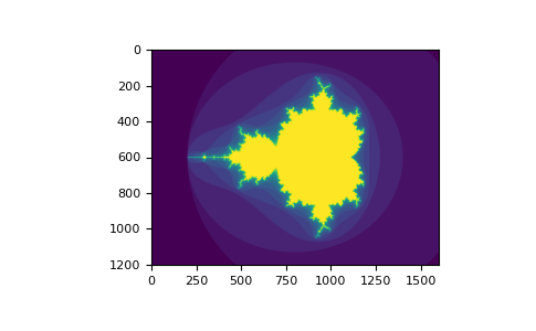
你可以通过下面的示例了解如何使用布尔数组来产生一个曼德罗伯集合的图像:
>>> import numpy as np
>>> import matplotlib.pyplot as plt
>>> def mandelbrot( h,w, maxit=20 ):
...     """Returns an image of the Mandelbrot fractal of size (h,w)."""
...     y,x = np.ogrid[ -1.4:1.4:h*1j, -2:0.8:w*1j ]
...     c = x+y*1j
...     z = c
...     divtime = maxit + np.zeros(z.shape, dtype=int)
...
...     for i in range(maxit):
...         z = z**2 + c
...         diverge = z*np.conj(z) > 2**2            # who is diverging
...         div_now = diverge & (divtime==maxit)  # who is diverging now
...         divtime[div_now] = i                  # note when
...         z[diverge] = 2                        # avoid diverging too much
...
...     return divtime
>>> plt.imshow(mandelbrot(400,400))
>>> plt.show()
第二个使用布尔量来进行索引的方法和常数索引更为类似。对于每一个维度我们提供一个一维数组来选出我们想要的部分:
>>> a = np.arange(12).reshape(3,4)
>>> b1 = np.array([False,True,True])             # first dim selection
>>> b2 = np.array([True,False,True,False])       # second dim selection
>>>
>>> a[b1,:]                                   # selecting rows
array([[ 4,  5,  6,  7],
       [ 8,  9, 10, 11]])
>>>
>>> a[b1]                                     # same thing
array([[ 4,  5,  6,  7],
       [ 8,  9, 10, 11]])
>>>
>>> a[:,b2]                                   # selecting columns
array([[ 0,  2],
       [ 4,  6],
       [ 8, 10]])
>>>
>>> a[b1,b2]                                  # a weird thing to do
array([ 4, 10])
注意,以为布尔数组的长度必须要你想要进行分片的部分长度相等。在之前的例子中,b1的长度为3(a的行数),b2(长度为4)可以用来索引a的第二个坐标轴(列)。
函数ix_()
函数ix_()可以将两个不同的向量结合来获得一个多元组的结果。例如,如果你想要对于a, b, c的每个元素及孙 a + b * c:
>>> a = np.array([2,3,4,5])
>>> b = np.array([8,5,4])
>>> c = np.array([5,4,6,8,3])
>>> ax,bx,cx = np.ix_(a,b,c)
>>> ax
array([[[2]],
       [[3]],
       [[4]],
       [[5]]])
>>> bx
array([[[8],
        [5],
        [4]]])
>>> cx
array([[[5, 4, 6, 8, 3]]])
>>> ax.shape, bx.shape, cx.shape
((4, 1, 1), (1, 3, 1), (1, 1, 5))
>>> result = ax+bx*cx
>>> result
array([[[42, 34, 50, 66, 26],
        [27, 22, 32, 42, 17],
        [22, 18, 26, 34, 14]],
       [[43, 35, 51, 67, 27],
        [28, 23, 33, 43, 18],
        [23, 19, 27, 35, 15]],
       [[44, 36, 52, 68, 28],
        [29, 24, 34, 44, 19],
        [24, 20, 28, 36, 16]],
       [[45, 37, 53, 69, 29],
        [30, 25, 35, 45, 20],
        [25, 21, 29, 37, 17]]])
>>> result[3,2,4]
17
>>> a[3]+b[2]*c[4]
17
你也可以按照下面的方法实现缩减:
>>> def ufunc_reduce(ufct, *vectors):
...    vs = np.ix_(*vectors)
...    r = ufct.identity
...    for v in vs:
...        r = ufct(r,v)
...    return r
然后这么使用上函数:
>>> ufunc_reduce(np.add,a,b,c)
array([[[15, 14, 16, 18, 13],
        [12, 11, 13, 15, 10],
        [11, 10, 12, 14,  9]],
       [[16, 15, 17, 19, 14],
        [13, 12, 14, 16, 11],
        [12, 11, 13, 15, 10]],
       [[17, 16, 18, 20, 15],
        [14, 13, 15, 17, 12],
        [13, 12, 14, 16, 11]],
       [[18, 17, 19, 21, 16],
        [15, 14, 16, 18, 13],
        [14, 13, 15, 17, 12]]])
相较于一般的 ufunc.reduce,这样做的好处是它充分利用了广播的性质来辩面创建一个输出大小乘以向量数量的参数数组。
字符串索引
线性代数
工作中基础的线性代数如下所示。
简单的数组操作
在numpy中的linalg.py了解更多
>>> import numpy as np
>>> a = np.array([[1.0, 2.0], [3.0, 4.0]])
>>> print(a)
[[ 1.  2.]
[ 3.  4.]]

>>> a.transpose()
array([[ 1.,  3.],
      [ 2.,  4.]])

>>> np.linalg.inv(a)
array([[-2. ,  1. ],
      [ 1.5, -0.5]])

>>> u = np.eye(2) # unit 2x2 matrix; "eye" represents "I"
>>> u
array([[ 1.,  0.],
      [ 0.,  1.]])
>>> j = np.array([[0.0, -1.0], [1.0, 0.0]])

>>> j @ j        # matrix product
array([[-1.,  0.],
      [ 0., -1.]])

>>> np.trace(u)  # trace
2.0

>>> y = np.array([[5.], [7.]])
>>> np.linalg.solve(a, y)
array([[-3.],
      [ 4.]])

>>> np.linalg.eig(j)
(array([ 0.+1.j,  0.-1.j]), array([[ 0.70710678+0.j        ,  0.70710678-0.j        ],
      [ 0.00000000-0.70710678j,  0.00000000+0.70710678j]]))
Parameters:
    square matrix
Returns
    The eigenvalues, each repeated according to its multiplicity.
    The normalized (unit "length") eigenvectors, such that the
    column ``v[:,i]`` is the eigenvector corresponding to the
    eigenvalue ``w[i]`` .
技巧和提示
这里我们提供一些简短但有效的提示。
“自动”重塑
你可以忽略一个尺寸来重塑数组的维度,忽略的尺寸将会被自动推断出来:
>>> a = np.arange(30)
>>> a.shape = 2,-1,3  # -1 means "whatever is needed"
>>> a.shape
(2, 5, 3)
>>> a
array([[[ 0,  1,  2],
        [ 3,  4,  5],
        [ 6,  7,  8],
        [ 9, 10, 11],
        [12, 13, 14]],
       [[15, 16, 17],
        [18, 19, 20],
        [21, 22, 23],
        [24, 25, 26],
        [27, 28, 29]]])
向量堆砌
我们怎么样将一些大小相同的行向量创建成一个二维数组?在MATLAB中这很简单:如果x和y是两个长度相等的,你只需要写 m = [x;y]。在NumPy中,你需要根据你想从哪个维度堆叠来分别调用函数column_stack,dstack,hstack和vstack:
x = np.arange(0,10,2)                     # x=([0,2,4,6,8])
y = np.arange(5)                          # y=([0,1,2,3,4])
m = np.vstack([x,y])                      # m=([[0,2,4,6,8],
                                          #     [0,1,2,3,4]])
xy = np.hstack([x,y])                     # xy =([0,2,4,6,8,0,1,2,3,4])
维度超过二时,这些函数的逻辑可能会比较奇怪。
参考
Numpy for MATLAB users
柱状图
NumPy函数histogram接受一个数组并返回两个向量:数组的直方图和每个柱的向量。注意:matplotlib同样有一个用来绘制直方图的函数(称为hist,就像Matlab里面一样),但和NumPy的函数有所不同。主要的区别就是pylab.hist自动划出柱状图,而numpy.histogram仅仅是产生数据。
>>> import numpy as np
>>> import matplotlib.pyplot as plt
>>> # Build a vector of 10000 normal deviates with variance 0.5^2 and mean 2
>>> mu, sigma = 2, 0.5
>>> v = np.random.normal(mu,sigma,10000)
>>> # Plot a normalized histogram with 50 bins
>>> plt.hist(v, bins=50, density=1)       # matplotlib version (plot)
>>> plt.show()

>>> # Compute the histogram with numpy and then plot it
>>> (n, bins) = np.histogram(v, bins=50, density=True)  # NumPy version (no plot)
>>> plt.plot(.5*(bins[1:]+bins[:-1]), n)
>>> plt.show()

后记:之前没有做过翻译,不知道翻译有多难,现在知道了。由于时间比较匆忙,许多地方翻译的不到位,也有许多打字的错误,欢迎大家指出。也希望大家能够从这篇翻译中有所裨益。


 1401
1401

 被折叠的 条评论
为什么被折叠?
被折叠的 条评论
为什么被折叠?
 到【灌水乐园】发言


