import numpy as np
import matplotlib.pyplot as plt
# 导入线性回归库
from sklearn.linear_model import LinearRegression
# 定义损失函数 ( y - w * x - b ) **2
def cost(w , b , points):
sum_cost = 0
M = len(points)
for i in range(M):
x = points[i,0]
y = points[i,1]
sum_cost += ( y - w * x - b ) ** 2
return sum_cost
if __name__ == '__main__':
"""
Ordinary least squares Linear Regression.
LinearRegression fits a linear model with coefficients w = (w1, ..., wp)
to minimize the residual sum of squares between the observed targets in
the dataset, and the targets predicted by the linear approximation.
普通最小二乘线性回归。
线性回归拟合的线性模型的系数为w = (w1,…wp)
使观测目标间的残差平方和最小
数据集,和目标预测的线性逼近。
"""
lr = LinearRegression()
# 读取数据
points = np.genfromtxt("D:\projects\PythonProjects\PythonStudy\data.csv",delimiter=",")
x = points[:,0]
y = points[:,1]
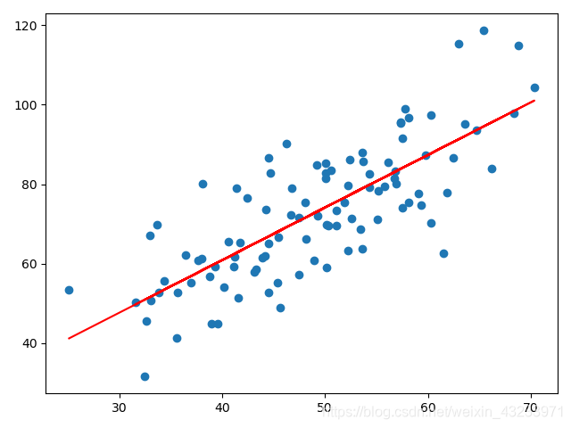
plt.scatter(x,y)
# 对 x, y 点进行转置 将一行n列的向量转换成n行一列的向量
new_x = x.reshape(-1,1)
new_y = y.reshape(-1,1)
# 根据训练数据集来得到模型
lr.fit(new_x,new_y)
w = lr.coef_[0][0]
b = lr.intercept_[0]
cost_list = cost(w,b,points)
print("w is :" ,w)
print("b is :" ,b)
print("cost_list is :" ,cost_list)
end_y = w * x + b
plt.plot(x , end_y , c = "r")
plt.show()
D:\Python\python.exe D:/projects/PythonProjects/PythonStudy/python-1/com/python/stuay/SkLearnLinearRegression.py
w is : 1.3224310227553597
b is : 7.991020982270399
cost_list is : 11025.738346621318
import numpy as npimport matplotlib.pyplot as plt# 导入线性回归库from sklearn.linear_model import LinearRegression# 定义损失函数 ( y - w * x - b ) **2def cost(w , b , points): sum_cost = 0 M = len(points) for i in range(M): x = points[i,0] .


 6839
6839


 被折叠的 条评论
为什么被折叠?
被折叠的 条评论
为什么被折叠?
 到【灌水乐园】发言


