MobileNet和HybridSN的学习

随风漂流l

于 2022-08-03 10:21:46 发布

阅读量822

点赞数

文章标签：深度学习 pytorch

本文链接：https://blog.csdn.net/weixin_43329973/article/details/126133289

版权

第4周学习：MobileNet+HybridSN

一、MobileNet
二、SE通道注意力机制
三、HybridSN
四、思考问题

一、MobileNet

该网络的主要亮点为，Depthwise Convolution（DW卷积），能大大减少参数和运算量；
增加两个参数一个是卷积层卷积核个数的超参数alpha，一个是控制输入图像大小的beta。专注于轻量级CNN网络，在准确率小幅下降的前提下，大大减少模型参数量和运算量。

mobileNet.V1
DW卷积，一个卷积核对应一个通道，所得到的out_channel==in_channel。在实际代码编写中，用group来表示，若group=1则表示普通卷积，若group=in_channel则表示DW卷积，若group=x则表示分组卷积。

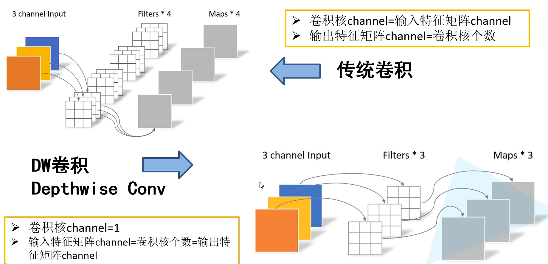
深度可分的卷积操作（depthwise separable Conv）由两部分组成，一个是DW卷积，一个是PW卷积（1x1卷积），将DW+PW运算量和普通卷积的运算量对比，理论上普通卷积计算量是深度可分卷积的8-9倍。网络计算量公式：K x K x inchannel x outchannel x input xinput。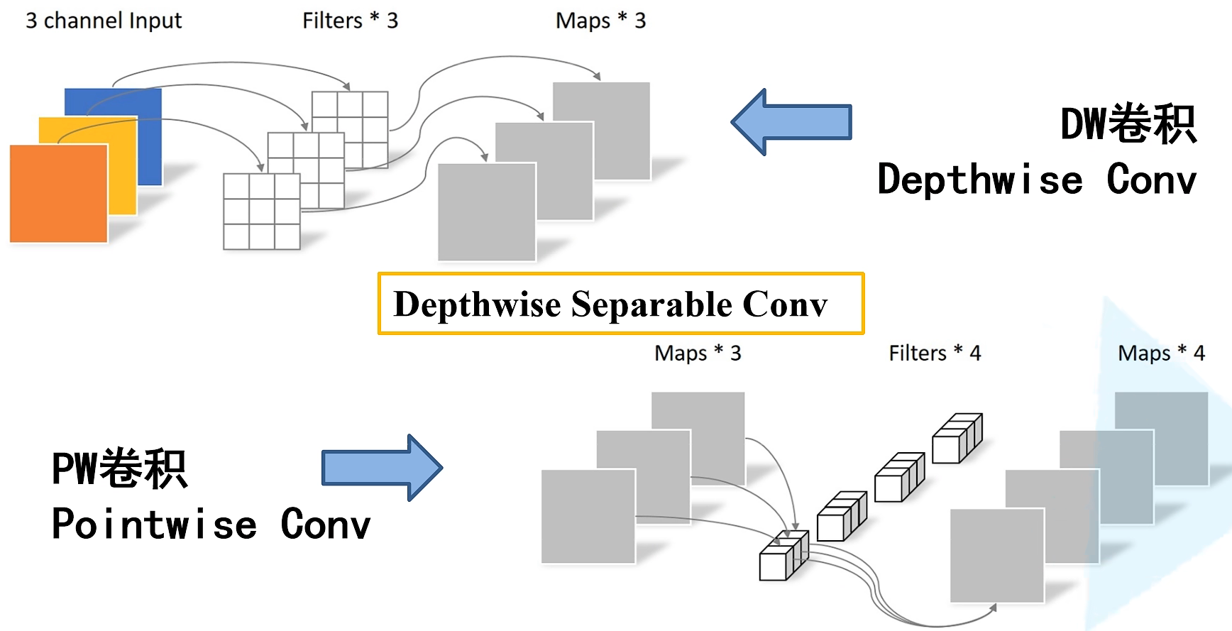
上述alpha与beta，alpha卷积核减少可以这么理解，因为好多卷积核并没有学到东西，所以卷积核深度没必要这么深；beta图像尺寸对准确率的影响。
mobileNet.V2
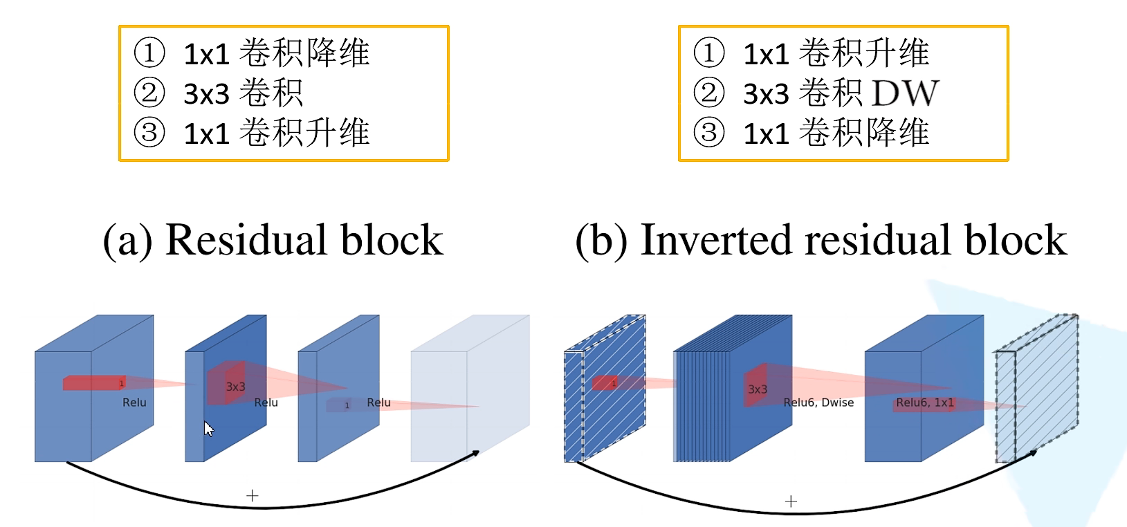
相较于V1版本，V2又加入了倒残差结构（inverted residual block），以及relu6激活函数。
首先我们看Inverted residual，DW卷积本身会造成信息损失，升维后再进行DW卷积可以减少信息损失，主要就是先升维再降维，激活函数的使用变为relu6。并且倒残差结构的最后一个1x1的卷积层使用的是线性激活函数，因为relu激活函数对低维特征信息会造成大量损失。最后要注意，当stride=1(说明卷积后尺寸不变）且输入与输出特征矩阵shape相同时才有shortcut连接。

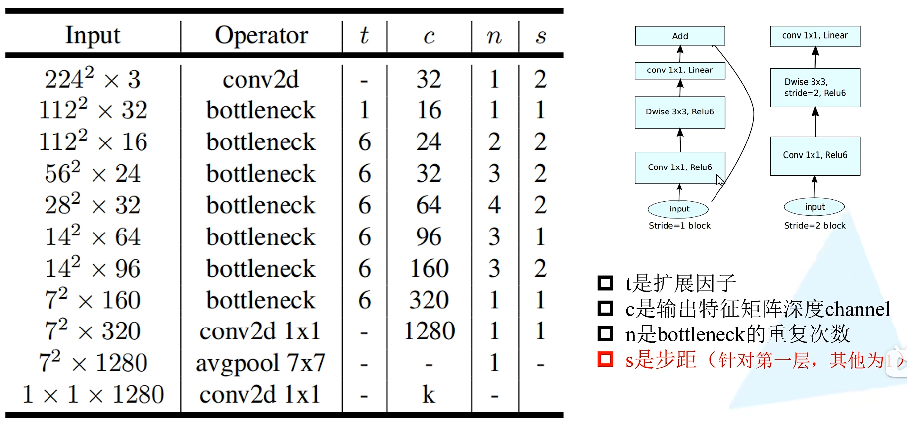
以下为具体的网络结构，并使用该结构进行分类预测。
注意，这里的s指的是每一层block第一个bottleneck的步距，其他默认为1。t指的是bottleneck中间升维的倍数expand_ratio。往往t=1那一层可以省略不写，因为使用的是1x1卷积核且只有深度发生了变化，影响不大。

附学习的v2网络结构，预训练模型下载地址：https://download.pytorch.org/models/mobilenet_v2-b0353104.pth
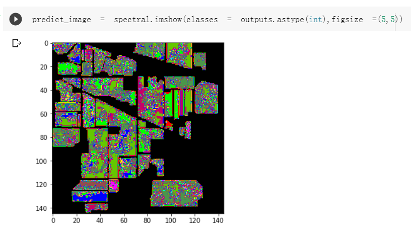
迭代5个epoch后的predict

from torch import nn
import torch
import torchvision.models.mobilenetv2

def _make_divisible(ch, divisor=8, min_ch=None):
    """
    This function is taken from the original tf repo.
    It ensures that all layers have a channel number that is divisible by 8
    It can be seen here:
    https://github.com/tensorflow/models/blob/master/research/slim/nets/mobilenet/mobilenet.py
    """
    if min_ch is None:
        min_ch = divisor
    new_ch = max(min_ch, int(ch + divisor / 2) // divisor * divisor)
    # Make sure that round down does not go down by more than 10%.
    if new_ch < 0.9 * ch:
        new_ch += divisor
    return new_ch


class ConvBNReLU(nn.Sequential):
    def __init__(self, in_channel, out_channel, kernel_size=3, stride=1, groups=1):
        padding = (kernel_size - 1) // 2
        super(ConvBNReLU, self).__init__(
            nn.Conv2d(in_channel, out_channel, kernel_size, stride, padding, groups=groups, bias=False),
            nn.BatchNorm2d(out_channel),
            nn.ReLU6(inplace=True)
        )


class InvertedResidual(nn.Module):
    def __init__(self, in_channel, out_channel, stride, expand_ratio):
        super(InvertedResidual, self).__init__()
        hidden_channel = in_channel * expand_ratio
        self.use_shortcut = stride == 1 and in_channel == out_channel

        layers = []
        if expand_ratio != 1:
            # 1x1 pointwise conv
            layers.append(ConvBNReLU(in_channel, hidden_channel, kernel_size=1))
        layers.extend([
            # 3x3 depthwise conv
            ConvBNReLU(hidden_channel, hidden_channel, stride=stride, groups=hidden_channel),
            # 1x1 pointwise conv(linear)
            nn.Conv2d(hidden_channel, out_channel, kernel_size=1, bias=False),
            nn.BatchNorm2d(out_channel),
        ])

        self.conv = nn.Sequential(*layers)

    def forward(self, x):
        if self.use_shortcut:
            return x + self.conv(x)
        else:
            return self.conv(x)


class MobileNetV2(nn.Module):
    def __init__(self, num_classes=1000, alpha=1.0, round_nearest=8):
        super(MobileNetV2, self).__init__()
        block = InvertedResidual
        input_channel = _make_divisible(32 * alpha, round_nearest)
        last_channel = _make_divisible(1280 * alpha, round_nearest)

        inverted_residual_setting = [
            # t, c, n, s
            [1, 16, 1, 1],
            [6, 24, 2, 2],
            [6, 32, 3, 2],
            [6, 64, 4, 2],
            [6, 96, 3, 1],
            [6, 160, 3, 2],
            [6, 320, 1, 1],
        ]

        features = []
        # conv1 layer
        features.append(ConvBNReLU(3, input_channel, stride=2))
        # building inverted residual residual blockes
        for t, c, n, s in inverted_residual_setting:
            output_channel = _make_divisible(c * alpha, round_nearest)
            for i in range(n):
                stride = s if i == 0 else 1 #每一层block第一个bottleneck的步距，其他默认为1
                features.append(block(input_channel, output_channel, stride, expand_ratio=t))
                input_channel = output_channel
        # building last several layers
        features.append(ConvBNReLU(input_channel, last_channel, 1))
        # combine feature layers
        self.features = nn.Sequential(*features)

        # building classifier
        self.avgpool = nn.AdaptiveAvgPool2d((1, 1))
        self.classifier = nn.Sequential(
            nn.Dropout(0.2),
            nn.Linear(last_channel, num_classes)
        )

        # weight initialization
        for m in self.modules():
            if isinstance(m, nn.Conv2d):
                nn.init.kaiming_normal_(m.weight, mode='fan_out')
                if m.bias is not None:
                    nn.init.zeros_(m.bias)
            elif isinstance(m, nn.BatchNorm2d):
                nn.init.ones_(m.weight)
                nn.init.zeros_(m.bias)
            elif isinstance(m, nn.Linear):
                nn.init.normal_(m.weight, 0, 0.01)
                nn.init.zeros_(m.bias)

    def forward(self, x):
        x = self.features(x)
        x = self.avgpool(x)
        x = torch.flatten(x, 1)
        x = self.classifier(x)
        return x

mobileNet.V3
相较于V2版本，主要是加入了注意力机制。并且重新设计了激活函数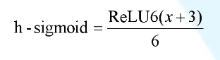，优化了量化过程。

二、SE通道注意力机制

Squeeze-and-Excitation Networks ，从特征通道的层面去考虑提升网络性能。
在这里插入图片描述
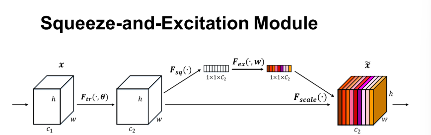
首先是Squeeze操作，为上图所示小白色矩形，将每个二维的特征通道变成一个实数，这个实数某种程度上具有全局的感受野，并且输出的维度和输入的特征通道数相匹配。

 # Squeeze 操作：global average pooling
        w = F.avg_pool2d(out, out.size(2))

其次是Excitation 操作。

 # 在 excitation 的两个全连接
        self.fc1 = nn.Conv2d(out_channels, out_channels//16, kernel_size=1) 
        self.fc2 = nn.Conv2d(out_channels//16, out_channels, kernel_size=1)
 #定义foward时
 # Excitation 操作： fc（压缩到16分之一）--Relu--fc（激到之前维度）--Sigmoid（保证输出为 0 至 1 之间）
        w = F.relu(self.fc1(w))
        w = F.sigmoid(self.fc2(w))

最后是一个Reweight的操作，我们将Excitation的输出的权重看做是进过特征选择后的每个特征通道的重要性，然后通过乘法逐通道加权到先前的特征上，完成在通道维度上的对原始特征的重标定。

# 重标定操作： 将卷积后的feature map与 w 相乘
        out = out * w

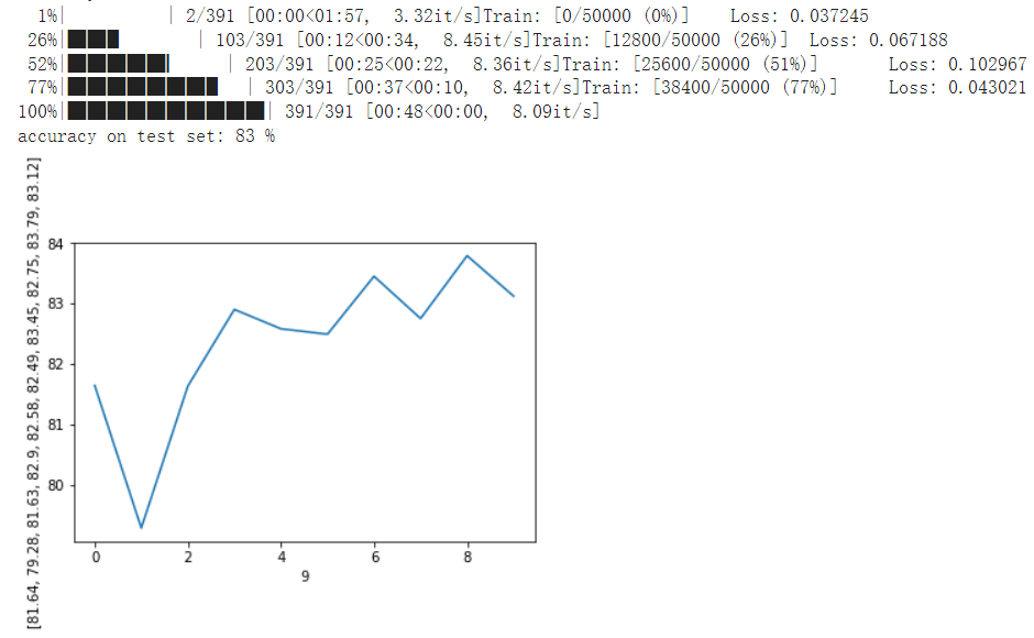
使用resnet18进行CIFAR10的分类预测，测试结果对比如下
在这里插入图片描述
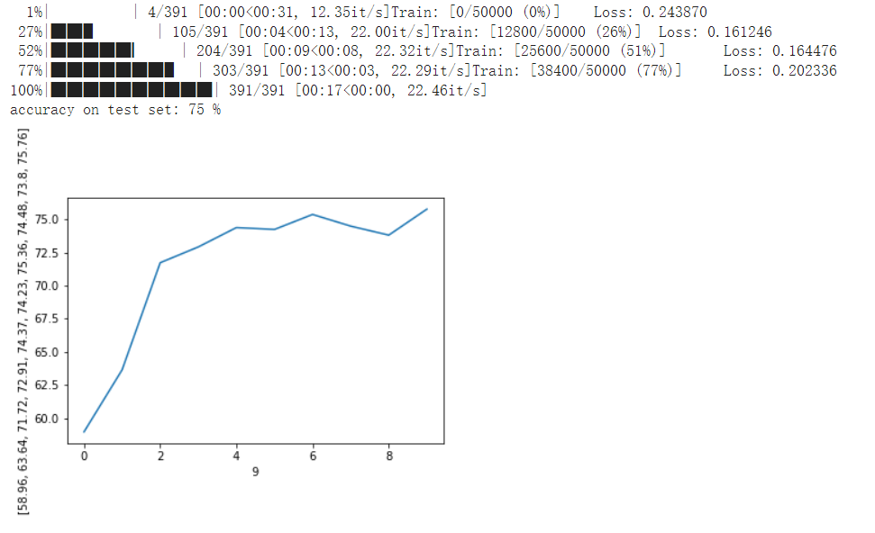
加入SE模块后的效果，可以看到有明显的效果提升。

三、HybridSN

论文学习
高光谱图像（HyperSpectral Image，简称HSI）

即包含光谱信息特别长的图像（包含红外线、紫外线等不可见光光谱），比如：普通照片只有三个通道，即RGB——红、绿、蓝。数据类型是一个m ∗ n ∗ 3的矩阵，而高光谱图像则是M ∗ N ∗ B （B是光谱的层数：3层RGB+其他光谱层…）。
高光谱图像是一个立体的三维结构，x、y表示二维平面像素信息坐标轴，第三维是波长信息坐标轴。
仅二维CNN无法从光谱维度中提取出具有良好鉴别能力的特征图。类似地，深度3D-CNN的计算更复杂，仅此一项似乎对在许多光谱带上具有类似纹理的类的性能更差。
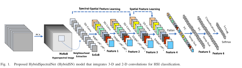
因此作者提出构建一种混合网络(HybridSN)解决了HSI分类所遇到的问题，它首先用三维CNN提取空间-光谱的特征，然后在三维CNN基础上进一步使用二维CNN学习更多抽象层次的空间特征，这与单独使用三维CNN相比，混合的CNN模型既降低了复杂性，也提升了性能。
HybridSN模型
HybridSN中可训练的权重参数总数为5122176，所有参数都是随机初始化的，使用Adam优化器，交叉熵损失函数，学习率为0.001，batch大小为256，训练100个epoch，抽取10%作为训练样本。结果还表明，所用的25×25空间维数最适合该方法。
为了首先消除谱冗余，传统的主成分分析（PCA）应用于原始HSI数据。主成分分析将光谱带的数量从D减少到B，同时保持相同的空间维度（即宽度M和高度N）。只减少了光谱带，从而保留了对识别任何物体都非常重要的空间信息。PCA大致原理讲解链接。

三维卷积部分：

conv1：（1, 30, 25, 25）， 8个 7x3x3 的卷积核 ==>（8, 24, 23, 23）
conv2：（8, 24, 23, 23）， 16个 5x3x3 的卷积核 ==>（16, 20, 21, 21）
conv3：（16, 20, 21, 21），32个 3x3x3 的卷积核 ==>（32, 18, 19, 19）
接下来要进行二维卷积，因此把前面的 32*18 reshape 一下，得到（576, 19, 19）

二维卷积：（576, 19, 19） 64个 3x3 的卷积核，得到（64, 17, 17）

接下来是一个 flatten 操作，变为 18496 维的向量，

接下来依次为256，128节点的全连接层，都使用比例为0.4的 Dropout，

最后输出为 16 个节点，是最终的分类类别数。
在这里插入图片描述

网络实现
下面是 HybridSN 类的代码：

class_num = 16
class HybridSN(nn.Module):
  def __init__(self):
    super(HybridSN,self).__init__()
    #根据论文计算，stride=1，padding=0
    self.conv1=nn.Conv3d(1,8,kernel_size=(7,3,3),stride=1,padding=0)
    #self.bn1=nn.BatchNorm3d(8)
    self.conv2=nn.Conv3d(8,16,kernel_size=(5,3,3),stride=1,padding=0)
    #self.bn2=nn.BatchNorm3d(16)
    self.conv3=nn.Conv3d(16,32,kernel_size=(3,3,3),stride=1,padding=0)
    #self.bn3=nn.BatchNorm3d(32)
    self.conv2D =nn.Conv2d(576,64,kernel_size=(3,3),stride=1,padding=0)
    #self.bn4=nn.BatchNorm3d(64)
    self.fc1=nn.Linear(18496,256)
    self.fc2=nn.Linear(256,128)
    self.fc3=nn.Linear(128,class_num)
    self.dropout=nn.Dropout(p=0.4)
    self.relu=nn.ReLU()

    #加入注意力机制,在 excitation 的两个全连接
    # self.SE=nn.Sequential(
    #     nn.Conv2d(576, 576//16, kernel_size=1),
    #     nn.ReLU(inplace=True),
    #     nn.Conv2d(576//16, 576, kernel_size=1),
    #     nn.Sigmoid()
    #     )

        
#self.soft = nn.LogSoftmax(dim=1) 能够解决函数overflow和underflow，加快运算速度，提高数据稳定性
  def forward(self,x):
    out = self.relu(self.conv1(x))
    out = self.relu(self.conv2(out))
    out = self.relu(self.conv3(out))
    #print("shape:",out.shape)
    #torch.Size([1, 32, 18, 19, 19])
    out = out.view(-1,out.shape[1]*out.shape[2],out.shape[3],out.shape[4])

    # w = F.avg_pool2d(out, out.size(2))
    # # Excitation 操作： fc（压缩到16分之一）--Relu--fc（激到之前维度）--Sigmoid（保证输出为 0 至 1 之间）
    # w = self.SE(out)
    # # 重标定操作： 将卷积后的feature map与 w 相乘，相当于恢复原尺寸
    # out = out * w 

    out = self.relu(self.conv2D(out))
    out = out.view(out.size(0),-1)
    out = self.dropout(self.fc1(out))
    out = self.dropout(self.fc2(out))
    out = self.fc3(out)
    return out
# 随机输入，测试网络结构是否通
x = torch.randn(1, 1, 30, 25, 25)
net = HybridSN()
y = net(x)
print(y.shape)

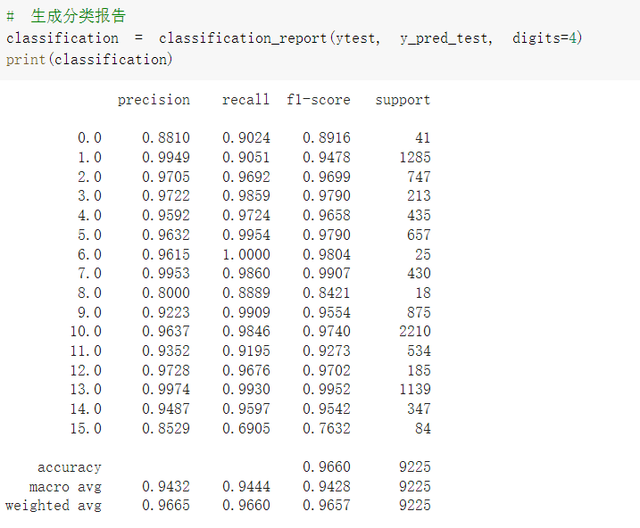
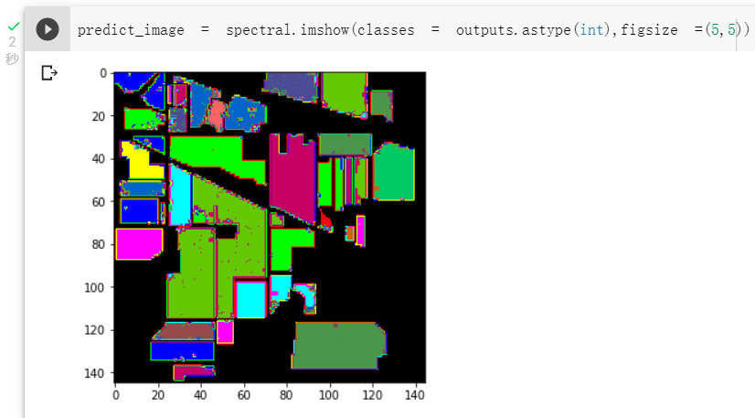
效果对比

原始网络结构，准确率为96.8%

- 加入注意力机制，准确率为92.08%，但可视化效果有所提升

- 加入BatchNormalization层，准确率提升为97.9%，该可视化效果可能是由于BN层将数据集中后所导致的。

四、思考问题

同一结构发现每次分类的结果都不一样，请思考为什么？
所有参数都是随机初始化的。可能是Dropout未关闭，model.eval()只能使得继承了nn.module的dropout失效，而不能使得自定义函数中的未继承module的dropout失效，增加了随机性，提供的源代码中也没有model.eval()和model.train()。
如果想要进一步提升高光谱图像的分类性能，可以如何改进？
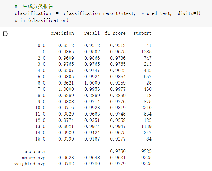
如上述分类效果所示，在2D卷积之前加入通道注意力模块，准确率有所下降，但视觉效果提升；加入BN层后，从收敛速度上看，HybridSN_BN快于另外两种模型，并且提升了模型分类准确度。