


深度学习(16)TensorFlow高阶操作五: 张量限幅
Outline
- clip_by_value
- relu
- clip_by_norm
- gradient clipping
1. clip_by_value
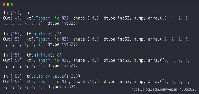
(1) tf.maximum(a, 2): 将a中比2小的数进行限幅,也就是比2小的全部变为2;
(2) tf.minimum(a, 8): 将a中比8大的数进行限幅,也就是比8大的全部变为8;
(3) tf.clip_by_value(a, 2, 8): 将a中比2小比8大的数进行限幅; 也就是比2小的全部变为2,比8大的全部变为8;
2. relu
当值小于0时,将值置位0; 当值大于0时,等于原值。
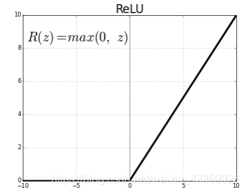
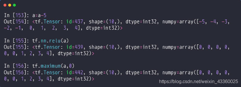
(1) tf.nn.relu(a): 将a进行relu化操作;
(2) tf.maximum(a, 0): 作用与tf.nn.relu(a)一样;
3. clip_by_norm
如果我们将一些数值限幅在我们希望的区域内,但是可能会导致梯度变化,就是不是我们希望看到的结果,这时我们就需要clip_by_norm()函数了,clip_by_norm的思想就是先求这个范围的向量值,也就是二范数,将其值限制在[0~1]之间,再放大这个范围,利用这个方法进行限幅就不会改变梯度值的大小。
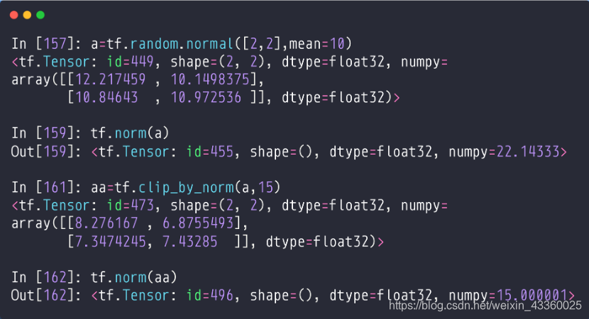
(1) tf.norm(a): 求a的二范数,即: √(∑▒x_i^2 );
(2) aa = tf.clip_by_norm(a, 15): 将a限制在15之间,但不改变其梯度大小,其中15就是一个new norm;
4. Gradient clipping
- Gradient Exploding or vanishing
- set lr=1
- new_grads, total_norm = tf.clip_by_global_norm(grads, 25)
目的在于保持整体的参数梯度方向不变,例如原来的
[
w
1
,
w
2
,
w
3
]
=
[
2
,
4
,
8
]
[w_1,w_2,w_3 ]=[2,4,8]
[w1,w2,w3]=[2,4,8],利用
clip_by_global_norm可以使
w
1
,
w
2
,
w
3
w_1,w_2,w_3
w1,w2,w3同时缩小n倍,例如同时缩小2倍,就是
[
w
1
,
w
2
,
w
3
]
=
[
1
,
2
,
4
]
[w_1,w_2,w_3 ]=[1,2,4]
[w1,w2,w3]=[1,2,4],这样就保证了梯度的方向不会发生变化。其中25代表梯度的值不会超过25。
5. 梯度爆炸实例以及利用clip_by_global_norm解决问题
(1) Before
我们为了演示梯度爆炸将学习率设置得高一点,这样即使是简单的MNIST数据集也会发生梯度爆炸问题。
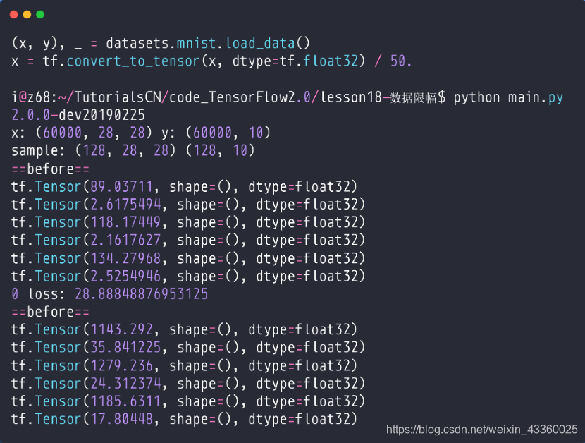
Step0: 我们可以看到(g-x代表x的梯度):
g-
w
1
w_1
w1=89.03711
g-
b
1
b_1
b1=2.6179454
g-
w
2
w_2
w2=118.17449
g-
b
2
b_2
b2=2.1617627
g-
w
3
w_3
w3=134.27968
g-
b
3
b_3
b3=2.5254946
Step1:
g-
w
1
w_1
w1=1143.292
g-
b
1
b_1
b1=35.148225
g-
w
2
w_2
w2=1279.236
g-
b
2
b_2
b2=24.312374
g-
w
3
w_3
w3=1185.6311
g-
b
3
b_3
b3=17.80448
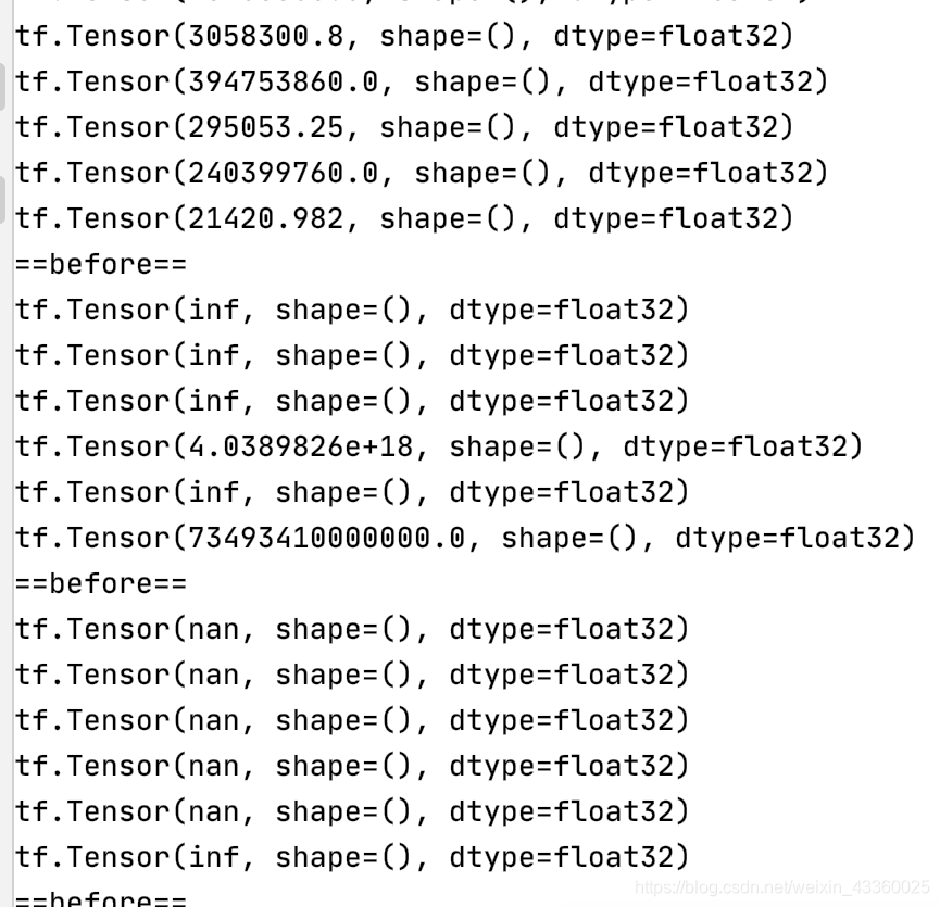
- 一般来说,梯度值在[0~20]之间我们是可以接受的,所以从第1轮训练之后就发生了Gradient Exploding(梯度爆炸)问题;
(2) Gradient Clipping
将
w
1
,
b
1
,
w
2
,
b
2
,
w
3
,
b
3
w_1,b_1,w_2,b_2,w_3,b_3
w1,b1,w2,b2,w3,b3通过clip_by_global_norm进行同比例裁剪; 15表示梯度值不会超过15;
(3) After
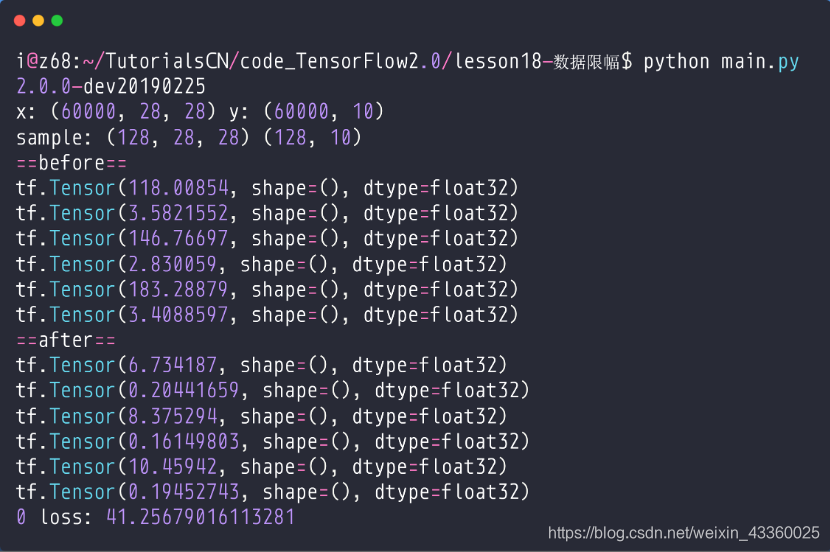
可以看到: 梯度相比于没有优化之前好了很多,这样我们在更新的时候是比较稳定的。
6. 实战
(1) Before
import tensorflow as tf
from tensorflow import keras
from tensorflow.keras import datasets, layers, optimizers
import os
os.environ['TF_CPP_MIN_LOG_LEVEL'] = '2'
print(tf.__version__)
(x, y), _ = datasets.mnist.load_data()
x = tf.convert_to_tensor(x, dtype=tf.float32) / 50.
y = tf.convert_to_tensor(y)
y = tf.one_hot(y, depth=10)
print('x:', x.shape, 'y:', y.shape)
train_db = tf.data.Dataset.from_tensor_slices((x, y)).batch(128).repeat(30)
x, y = next(iter(train_db))
print('sample:', x.shape, y.shape)
# print(x[0], y[0])
def main():
# 784 => 512
w1, b1 = tf.Variable(tf.random.truncated_normal([784, 512], stddev=0.1)), tf.Variable(tf.zeros([512]))
# 512 => 256
w2, b2 = tf.Variable(tf.random.truncated_normal([512, 256], stddev=0.1)), tf.Variable(tf.zeros([256]))
# 256 => 10
w3, b3 = tf.Variable(tf.random.truncated_normal([256, 10], stddev=0.1)), tf.Variable(tf.zeros([10]))
optimizer = optimizers.SGD(lr=0.01)
for step, (x, y) in enumerate(train_db):
# [b, 28, 28] => [b, 784]
x = tf.reshape(x, (-1, 784))
with tf.GradientTape() as tape:
# layer1.
h1 = x @ w1 + b1
h1 = tf.nn.relu(h1)
# layer2
h2 = h1 @ w2 + b2
h2 = tf.nn.relu(h2)
# output
out = h2 @ w3 + b3
# out = tf.nn.relu(out)
# compute loss
# [b, 10] - [b, 10]
loss = tf.square(y - out)
# [b, 10] => [b]
loss = tf.reduce_mean(loss, axis=1)
# [b] => scalar
loss = tf.reduce_mean(loss)
# compute gradient
grads = tape.gradient(loss, [w1, b1, w2, b2, w3, b3])
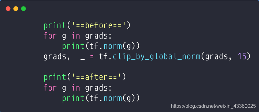
print('==before==')
for g in grads:
print(tf.norm(g))
# grads, _ = tf.clip_by_global_norm(grads, 15)
# print('==after==')
# for g in grads:
# print(tf.norm(g))
# update w' = w - lr*grad
optimizer.apply_gradients(zip(grads, [w1, b1, w2, b2, w3, b3]))
if step % 100 == 0:
print(step, 'loss:', float(loss))
if __name__ == '__main__':
main()
注: 这里因为很难出现梯度爆炸的问题,为了实验clip_by_global_norm方法的效率,我们将原数据集输入除以50,以达到梯度爆炸的效果。
运行结果如下:
(2) After
import tensorflow as tf
from tensorflow import keras
from tensorflow.keras import datasets, layers, optimizers
import os

os.environ['TF_CPP_MIN_LOG_LEVEL'] = '2'
print(tf.__version__)

(x, y), _ = datasets.mnist.load_data()
x = tf.convert_to_tensor(x, dtype=tf.float32) / 50.
y = tf.convert_to_tensor(y)
y = tf.one_hot(y, depth=10)
print('x:', x.shape, 'y:', y.shape)
train_db = tf.data.Dataset.from_tensor_slices((x, y)).batch(128).repeat(30)
x, y = next(iter(train_db))
print('sample:', x.shape, y.shape)


# print(x[0], y[0])


def main():
    # 784 => 512
    w1, b1 = tf.Variable(tf.random.truncated_normal([784, 512], stddev=0.1)), tf.Variable(tf.zeros([512]))
    # 512 => 256
    w2, b2 = tf.Variable(tf.random.truncated_normal([512, 256], stddev=0.1)), tf.Variable(tf.zeros([256]))
    # 256 => 10
    w3, b3 = tf.Variable(tf.random.truncated_normal([256, 10], stddev=0.1)), tf.Variable(tf.zeros([10]))

    optimizer = optimizers.SGD(lr=0.01)

    for step, (x, y) in enumerate(train_db):

        # [b, 28, 28] => [b, 784]
        x = tf.reshape(x, (-1, 784))

        with tf.GradientTape() as tape:

            # layer1.
            h1 = x @ w1 + b1
            h1 = tf.nn.relu(h1)
            # layer2
            h2 = h1 @ w2 + b2
            h2 = tf.nn.relu(h2)
            # output
            out = h2 @ w3 + b3
            # out = tf.nn.relu(out)

            # compute loss
            # [b, 10] - [b, 10]
            loss = tf.square(y - out)
            # [b, 10] => [b]
            loss = tf.reduce_mean(loss, axis=1)
            # [b] => scalar
            loss = tf.reduce_mean(loss)

        # compute gradient
        grads = tape.gradient(loss, [w1, b1, w2, b2, w3, b3])
        print('==before==')
        for g in grads:
            print(tf.norm(g))

        grads, _ = tf.clip_by_global_norm(grads, 15)

        print('==after==')
        for g in grads:
            print(tf.norm(g))
        # update w' = w - lr*grad
        optimizer.apply_gradients(zip(grads, [w1, b1, w2, b2, w3, b3]))

        if step % 100 == 0:
            print(step, 'loss:', float(loss))


if __name__ == '__main__':
    main()
运行结果如下:
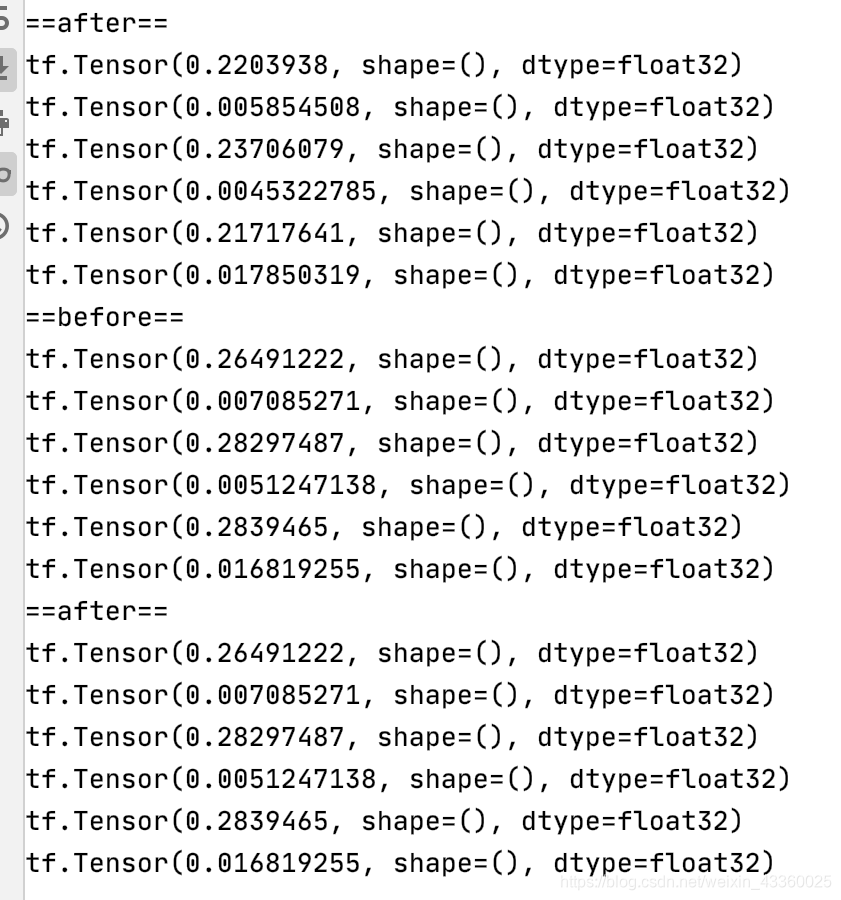
可以看到,即使迭代了几十轮,这些参数还是能够在正常范围内进行更新。
(3) 查看收敛
import tensorflow as tf
from tensorflow import keras
from tensorflow.keras import datasets, layers, optimizers
import os

os.environ['TF_CPP_MIN_LOG_LEVEL'] = '2'
print(tf.__version__)

(x, y), _ = datasets.mnist.load_data()
x = tf.convert_to_tensor(x, dtype=tf.float32) / 50.
y = tf.convert_to_tensor(y)
y = tf.one_hot(y, depth=10)
print('x:', x.shape, 'y:', y.shape)
train_db = tf.data.Dataset.from_tensor_slices((x, y)).batch(128).repeat(30)
x, y = next(iter(train_db))
print('sample:', x.shape, y.shape)


# print(x[0], y[0])


def main():
    # 784 => 512
    w1, b1 = tf.Variable(tf.random.truncated_normal([784, 512], stddev=0.1)), tf.Variable(tf.zeros([512]))
    # 512 => 256
    w2, b2 = tf.Variable(tf.random.truncated_normal([512, 256], stddev=0.1)), tf.Variable(tf.zeros([256]))
    # 256 => 10
    w3, b3 = tf.Variable(tf.random.truncated_normal([256, 10], stddev=0.1)), tf.Variable(tf.zeros([10]))

    optimizer = optimizers.SGD(lr=0.01)

    for step, (x, y) in enumerate(train_db):

        # [b, 28, 28] => [b, 784]
        x = tf.reshape(x, (-1, 784))

        with tf.GradientTape() as tape:

            # layer1.
            h1 = x @ w1 + b1
            h1 = tf.nn.relu(h1)
            # layer2
            h2 = h1 @ w2 + b2
            h2 = tf.nn.relu(h2)
            # output
            out = h2 @ w3 + b3
            # out = tf.nn.relu(out)

            # compute loss
            # [b, 10] - [b, 10]
            loss = tf.square(y - out)
            # [b, 10] => [b]
            loss = tf.reduce_mean(loss, axis=1)
            # [b] => scalar
            loss = tf.reduce_mean(loss)

        # compute gradient
        grads = tape.gradient(loss, [w1, b1, w2, b2, w3, b3])
        # print('==before==')
        # for g in grads:
        #     print(tf.norm(g))

        grads, _ = tf.clip_by_global_norm(grads, 15)

        # print('==after==')
        # for g in grads:
        #     print(tf.norm(g))
        # update w' = w - lr*grad
        optimizer.apply_gradients(zip(grads, [w1, b1, w2, b2, w3, b3]))

        if step % 100 == 0:
            print(step, 'loss:', float(loss))


if __name__ == '__main__':
    main()
运行结果如下:
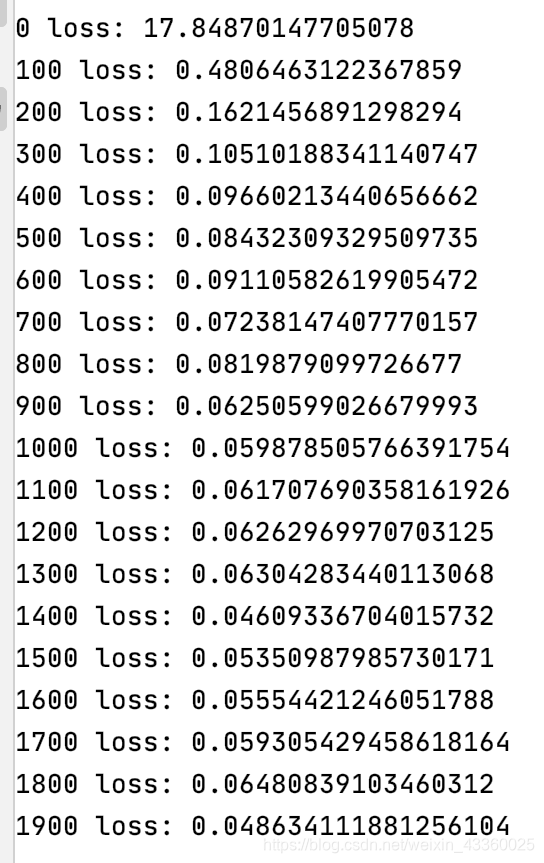
可以看到,模型能够很好地收敛。
参考文献:
[1] 龙良曲:《深度学习与TensorFlow2入门实战》


 1083
1083


 被折叠的 条评论
为什么被折叠?
被折叠的 条评论
为什么被折叠?
 到【灌水乐园】发言


