


1.张量 tensor
(1) torch.tensor
(data,
dtype=None,
device=None,
requires_grad=False,
pin_memory=False) # pin_memory是否存于锁页内存
(2) torch.from_numpy(ndarray)
【注】tensor和ndarray共享内存
(3) torch.zeros
(*size,
out=None,
dtype=None,
layout=torch.strided,
device=None,
requires_grad=False) 依size创建全0的张量
torch.zeros_like(input,
				dtype=None,
				device=None,
				requires_grad=False) 依input形状创建全0的张量
(4) torch.ones
(*size,
out=None,
dtype=None,
layout=torch.strided,
device=None,
requires_grad=False)
torch.ones_like(input,
				dtype=None,
				layout=None,
				device=None,
				requires_grad=False) 依input形状创建全1的张量
(5) torch.linspace
(start,
end,
steps=100,
out=None,
dtype=None,
layout=torch.strided,
device=None,
requires_grad=False) 创建均分的1维张量
(6) torch.logspace
(start,
end,
steps=100,
base=10.0,
out=None,
dtype=None,
layout=torch.strided,
device=None,
requires_grad=False) 创建对数均分的1维张量
(7) torch.eye
(n.
m=None,
out=None,
dtype=None,
layout=torch.strided,
device=None,
requires_grad=False) 创建单位对角矩阵
(8) torch.normal(mean, std, size, out=None)
生成正态分布 (即:高斯分布)
(9) torch.randn
(*size,
out=None,
dtype=None,
layout=torch.strided,
device=None,
requires_grad=False) 生成标准正态分布
torch.randn_like()
(10) torch.rand
(*size,
out=None,
dtype=None,
layout=torch.strided,
device=None,
requires_grad=False) 在区间[0,1)上生成均匀分布
torch.rand_like()
(11) torch.randint
(*size,
out=None,
dtype=None,
layout=torch.strided,
device=None,
requires_grad=False) 在区间[low,high)上生成整数均匀分布
torch.randint_like()
(12) torch.randperm
(n,
out=None,
dtype=None,
layout=torch.strided,
device=None,
requires_grad=False) 生成从0到n-1的随机排列
(13) torch.bernoulli(input, *, generator=None, out=None)
以input为概率,生成伯努利分布(0-1分布,两点分布) # input是概率值
2.张量的操作
(1) torch.cat
(tensors,
dim=0,
out=None) 将张量按维度dim进行拼接 # tensors张量序列
(2) torch.stack
(tensors,
dim=0,
out=None) 在新创建的维度dim上进行拼接
(3) torch.chunk
(input,
chunks,
dim=0) 将张量按维度dim进行平均切分 # chunks要切分的份数;若不能整除均分,最后一份张量小于其他张量
(4) torch.split
(tensor,
split_size_or_sections,
dim=0) 将张量按维度dim进行切分 # split_size_or_sections为int或者list
(5) torch.index_select
(input,
dim,
index,
out=None) 在维度dim上,按index索引数据
(6) torch.mask_select
(input,
mask,
out=None) 按mask的True进行索引
(7) torch.reshape(input, shape)
变换张量形状 # 注意:当张量在内存中是连续时,新张量与input共享数据内存
(8) torch.transpose(input, dim0, dim1) 交换张量的两个维度
torch.t() 2维张量转置,对矩阵而言,等价于torch.transpose(input, 0, 1)
(9) torch.squeeze(input, dim=None, out=None)
压缩长度为1的维度 # 如果dim为None,则移除所有长度为1的轴,若指定维度,当且仅当该轴长度为1时,可以被移除;
torch.unsqueeze(input, dim, out=None) 依据dim扩展维度
(10) 加减乘除
torch.add(input, alpha=1, other, out=None)
torch.addcdiv(input, value=1, tensor1, tensor2, out=None)
torch.addcmul(input, value=1, tensor1, tensor2, out=None)
torch.sub()
torch.div()
torch.mul()
torch.log()
torch.log10()
torch.log2()
torch.exp()
torch.pow()
torch.abs()
torch.cos()
…
3.计算图与动态图机制
(1)计算图的定义:计算图是用来描述运算的有向无环图,两个主要因素:结点和边,结点表示数据(如:向量、矩阵、张量),边表示运算(如:加减乘数卷积等);
(2)grad_fn:记录创建该张量时所用的方法;
(3)动态图与静态图的区别:静态图是先搭建图,后运算,特点高效但不灵活;而动态图是运算与搭建同时进行,特点灵活且易调节;
4. autograd自动求导
(1) 自动求导梯度:
	torch.autograd.backward
	(tensors,   # tensors: 用于求导的张量,如 loss
	grad_tensors=None,   # grad_tensors: 多梯度权重
	retain_grad=None,   # retain_graph: 保存计算图
	create_graph=False)    # create_graph: 创建导数计算图,用于高阶求导
(2) torch.autograd.grad
(outputs,
inputs,
grad_outputs=None,
retain_grad=None,
create_graph=False) 求梯度
【注】 梯度不会自动清零;依赖于叶子结点的结点requires_grad默认True;叶子结点不可以执行in-place;
5. 逻辑回归Logistic Regression
定义:逻辑回归是线性的二分类模型;
公式:
y=f(x)=1/(1+e^-x) —sigmoid函数,即:logistics函数
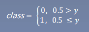

【注】 线性回归是分析自变量x与因变量y(标量)之间关系的方法;
逻辑回归是分析自变量x与因变量y(概率)之间关系的方法;


 5066
5066


 被折叠的 条评论
为什么被折叠?
被折叠的 条评论
为什么被折叠?
 到【灌水乐园】发言


