超参数的调优（lightgbm)

参考
原文
Automated Hyperparameter Optimization

超参数的优化过程：通过自动化
目的：使用带有策略的启发式搜索（informed search）在更短的时间内找到最优超参数，除了初始设置之外，并不需要额外的手动操作。

实践部分

贝叶斯优化问题有四个组成部分：

1. 目标函数：我们想要最小化的对象，这里指带超参数的机器学习模型的验证误差

2. 域空间：待搜索的超参数值

3. 优化算法：构造代理模型和选择接下来要评估的超参数值的方法

4. 结果的历史数据：存储下来的目标函数评估结果，包含超参数和验证损失

通过以上四个步骤，我们可以对任意实值函数进行优化（找到最小值）。这是一个强大的抽象过程，除了机器学习超参数的调优，它还能帮我们解决其他许多问题。

代码示例

数据集：https://www.jiqizhixin.com/articles/2018-08-08-2
目标：预测客户是否会购买一份保险产品
监督分类问题
观测值：5800
测试点：4000
不平衡的分类问题，本文使用的评价性能的指标是受试者工作特征曲线下的面积（ROC AUC），ROC AUC 的值越高越好，其值为 1 代表模型是完美的。

什么是不平衡的分类问题？
如何处理数据中的「类别不平衡」？
极端类别不平衡数据下的分类问题S01：困难与挑战

hyperropt1125.py

- 导入库

import pandas as pd
import numpy as np
import matplotlib.pyplot as plt
import seaborn as sns
import lightgbm as lgb
from sklearn.model_selection import KFold

MAX_EVALIS = 500
N_FLODS = 10

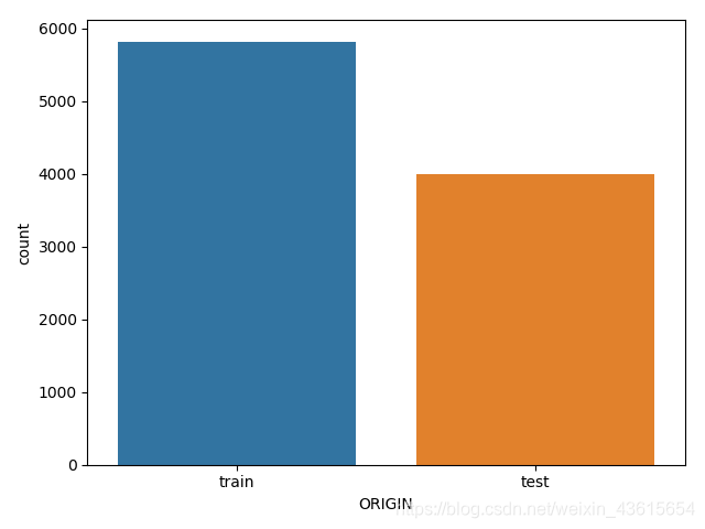
观察数据，数据集已经用ORIGIN把数据自动分为train和test集。

print(data.ORIGIN.value_counts())

train    5822
test     4000
Name: ORIGIN, dtype: int64

复习一下，随意画个图

sns.countplot(x='ORIGIN',data=data)
plt.show()

CARAVAN： target

- 处理数据集

一定要细心啊，不然BUG真的莫名其妙。

#导入后先划分训练集和测试集
train = data[data['ORIGIN'] == 'train']
test = data[data['ORIGIN'] == 'test']

#抽取标签
train_labels = np.array(train['CARAVAN'].astype(np.int32)).reshape((-1,))
test_labels = np.array(test['CARAVAN'].astype(np.int32)).reshape((-1,))

去掉标签们，留下特征
train = train.drop(columns = ['ORIGIN','CARAVAN'])
test = test.drop(columns = ['ORIGIN','CARAVAN'])

features = np.array(train)
test_features = np.array(test)
labels = train_labels[:]

print('Train shape: {}'.format(train.shape))
print("Test shape :{}".format(test.shape))
train.head()

#运行结果
Train shape: (5822, 85)
Test shape :(4000, 85)

Python中reshape函数参数-1的意思
不分行列，改成1串

- 标签分布

plt.hist(labels, edgecolor = 'k')
plt.xlabel('Label')
plt.ylabel('Count')
plt.title('Counts of Labels')

plt.show()

hist函数1

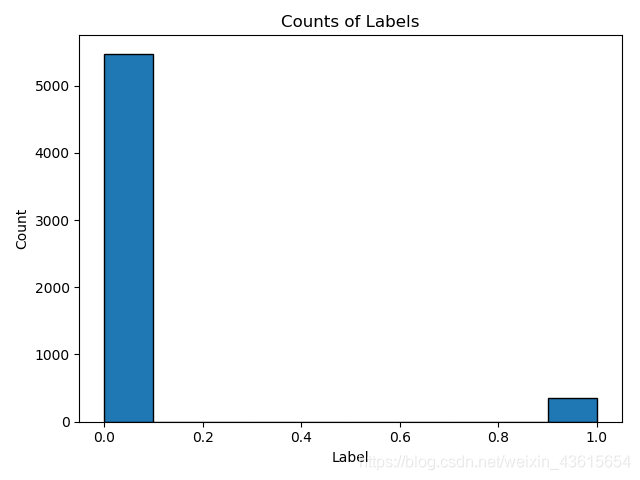
可以看出，这是个不平衡的分类问题。
因此，选用梯度提升模型，验证方法采用ROC AUC。（具体见原文了）
本文采用的是LightGBM。

-模型与其默认值

from lightgbm import LGBMClassifier
model = LGBMClassifier()#Model with default hyperparameters
print(model)

LGBMClassifier(boosting_type='gbdt', class_weight=None, colsample_bytree=1.0,
        importance_type='split', learning_rate=0.1, max_depth=-1,
        min_child_samples=20, min_child_weight=0.001, min_split_gain=0.0,
        n_estimators=100, n_jobs=-1, num_leaves=31, objective=None,
        random_state=None, reg_alpha=0.0, reg_lambda=0.0, silent=True,
        subsample=1.0, subsample_for_bin=200000, subsample_freq=0)

将模型与训练集拟合，采用roc_auc验证。

from sklearn.metrics import roc_auc_score
from timeit import default_timer as timer

start = timer()
model.fit(features,labels)
train_time = timer() - start

predictions = model.predict_proba(test_features)[:,1]
auc = roc_auc_score(test_labels,predictions)

print('The baseline score on the test set is {:.4f}.'.format(auc))
print('The baseline training time is {:.4f} seconds'.format(train_time))

#results
The baseline score on the test set is 0.7092.
The baseline training time is 0.1888 seconds

Due to the small size of the dataset (less than 6000 observations), hyperparameter tuning will have a modest but noticeable effect on the performance (a better investment of time might be to gather more data!)

python中计时工具timeit模块的基本用法
测试代码运行时间

Random Search

import random

随机搜索也有四个部分：

Domain: values over which to search
Optimization algorithm: pick the next values at random! (yes this qualifies as an algorithm)
Objective function to minimize: in this case our metric is cross validation ROC AUC
Results history that tracks the hyperparameters tried and the cross validation metric

让我们来康康哪些参数要Tuning

- Domain for Random Search

Random search and Bayesian optimization 都是从domain搜索hyperparameters，对于random (or grid search)，这种domain被称为hyperparameter grid，并且对hyperparameter使用离散值。

print(LGBMClassifier())

#Results
LGBMClassifier(boosting_type='gbdt', class_weight=None, colsample_bytree=1.0,
        importance_type='split', learning_rate=0.1, max_depth=-1,
        min_child_samples=20, min_child_weight=0.001, min_split_gain=0.0,
        n_estimators=100, n_jobs=-1, num_leaves=31, objective=None,
        random_state=None, reg_alpha=0.0, reg_lambda=0.0, silent=True,
        subsample=1.0, subsample_for_bin=200000, subsample_freq=0)

基于默认值，以下可构建hyperparameter grid。在此之前选值怎么工作得更好并不好说，因此对于大部分参数我们均采用默认值或以默认值为中心上下浮动的值。
**注意：**subsample_dist是subsample的参数，但boosting_type=goss不支持随机的 subsampling。
假如boosting_type选择其他值，那么这个subsample_dist可以放到param_grid里让我们随机搜索。

param_grid = {
    'class_weight': [None, 'balanced'],
    'boosting_type': ['gbdt', 'goss', 'dart'],
    'num_leaves': list(range(30, 150)),
    'learning_rate': list(np.logspace(np.log(0.005), np.log(0.2), base = np.exp(1), num = 1000)),
    'subsample_for_bin': list(range(20000, 300000, 20000)),
    'min_child_samples': list(range(20, 500, 5)),
    'reg_alpha': list(np.linspace(0, 1)),
    'reg_lambda': list(np.linspace(0, 1)),
    'colsample_bytree': list(np.linspace(0.6, 1, 10))
}

# Subsampling (only applicable with 'goss')
subsample_dist = list(np.linspace(0.5, 1, 100))

让我们来康康 learning_rate 和 the num_leaves的分布，学习率是典型的对数分布，参见Quora这篇Why does one sample the log-space when searching for good Hyper Parameters for Machine Learning

because it can vary over several orders of magnitude

因此，可以采用np.logspace 搜索。

np.logspace returns values evenly spaced over a log-scale (so if we take the log of the resulting values, the distribution will be uniform

plt.hist(param_grid['learning_rate'],color='g',edgecolor = 'k')
plt.xlabel('Learning Rate', size = 14)
plt.ylabel('Count', size = 14)
plt.title('Learning Rate Distribution', size = 18)
plt.show()

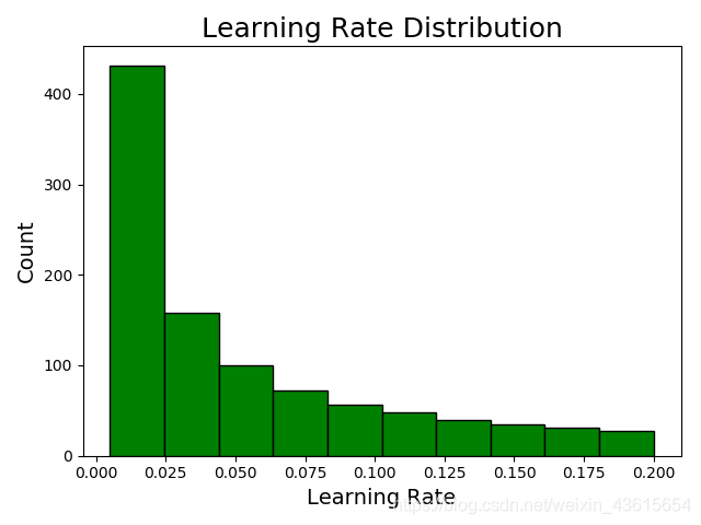
在0,005与0.2之间的值较多。建议在这个范围里选值。

再来看看num_leaves的表现

plt.hist(param_grid['num_leaves'], color = 'b', edgecolor = 'k')
plt.xlabel('Learning Number of Leaves', size = 14)
plt.ylabel('Count', size = 14)
plt.title('Number of Leaves Distribution', size = 18)
plt.show()

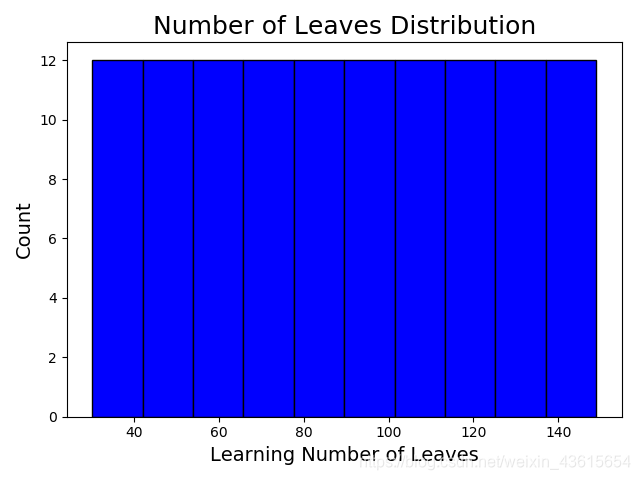
没什么波动。

-Sampling from Hyperparameter Domain

查看我们采样的结果：

params = {key:random.sample(value,1)[0] for key,value in param_grid.items()}
print(params)

#运行结果
{'class_weight': 'balanced', 'boosting_type': 'gbdt', 'num_leaves': 49, 'learning_rate': 0.006450936939768325, 'subsample_for_bin': 140000, 'min_child_samples': 145, 'reg_alpha': 0.16326530612244897, 'reg_lambda': 0.9387755102040816, 'colsample_bytree': 0.6444444444444444}

其他：
生成随机系数

import random
a = dict(....) # a is some dictionary
random_key = random.sample(a, 1)[0]

python 字典操作提取key,value

#!/usr/bin/env python3
# -*- coding: utf-8 -*-

dict_ori = {'A':1, 'B':2, 'C':3}
dict_new = {key:value for key,value in dict_ori.items()}
print(dict_new)

注意这句
‘boosting_type’: [‘gbdt’, ‘goss’, ‘dart’],
在 boosting_type 选择非 goss类型时，对subsample也能采取随机采样。

params['subsample'] = random.sample(subsample_dist, 1)[0] if params['boosting_type'] != 'goss' else 1.0
print(params)

#运行结果
{'class_weight': 'balanced', 'boosting_type': 'gbdt', 'num_leaves': 47, 'learning_rate': 0.008572448761425775, 'subsample_for_bin': 20000, 'min_child_samples': 420, 'reg_alpha': 0.6122448979591836, 'reg_lambda': 0.7142857142857142, 'colsample_bytree': 0.7333333333333333, 'subsample': 0.8282828282828283}

-Cross Validation with Early Stopping in LightGBM

使用LightGBM的cross validation function，采用100 early stopping rounds。
建立数据集，懒得改了，但是我的习惯是，features用X_train表达,labels用y_train = labels表达

train_set = lgb.Dataset(features,labels)
cv_results = lgb.cv(params,train_set,num_boost_round=10000,nfold=10,metrics='auc',early_stopping_rounds=100,verbose_eval=False,seed=50)
#最高分
cv_results_best = np.max(cv_results['auc-mean'])
#最高分的标准差
cv_results_std = cv_results['auc-stdv'][np.argmax(['auc-mean'])]

print("the maximum ROC AUC on the validation set was{:.5f} with std of {:.5f}.".format(cv_results_best,cv_results_std))
print('The ideal number of iteractions was {}.'.format(np.argmax(cv_results['auc-mean'])+1))

#运行结果
the maximum ROC AUC on the validation set was0.75260 with std of 0.03831.
The ideal number of iteractions was 5.

详解numpy的argmax
找出最大值的索引。即最好迭代步

之前的方法

print('best n_estimator is {}'.format(len(cv_results['auc-mean'])))
print('best cv score is {}'.format(pd.Series(cv_results['auc-mean']).max()))

#运行结果
best n_estimator is 7
best cv score is 0.7568251976593624

-Results Dataframe

从前面的运算，我们已经获取了：

• domain
• algorithm（还记得吗？选值的）
  另外还需要
  Objective function to minimize: in this case our metric is cross validation ROC AUC
  Results history that tracks the hyperparameters tried and the cross validation metric

Tracking the results 将通过一个dataframe完成，每行对目标函数进行评估。

random_results = pd.DataFrame(columns=['loss','params','iteration','estimator','time'],index=list(range(MAX_EVALIS)))

#index行标签

-目标函数

我们试图最小化目标函数。其输入为一组值——在本例中为 GBM 的超参数，输出为需要最小化的实值——交叉验证损失。Hyperopt
将目标函数作为黑盒处理，因为这个库只关心输入和输出是什么。为了找到使损失最小的输入值，该算法不需要知道目标函数的内部细节！

与从训练数据中提取验证集（从而限制我们拥有的训练数据的数量）相比，更好的方法是KFold交叉验证。

对于此示例，我们将使用10倍交叉验证，这意味着测试和训练每组模型超参数10次，每次使用不同的训练数据子集作为验证集。

在随机搜索的情况下，下一个选择的值不是基于过去的评估结果，但显然仍应对运算保持跟踪，以便我们知道哪个值最有效。 这也将使我们能够将随机搜索与明智的贝叶斯优化进行对比。

-Random Search Implementation随机搜索的实现

目的：写一个循环遍历评估次数，每次选择一组不同的超参数进行评估。
每次运行该函数，结果都会保存到dataframe中。

关于乱序（shuffle）与随机采样（sample）的一点探究

random.seed(50)
#用前面设置好的值来作为遍历的次数：
for i in range(MAX_EVALIS):
    params = {key:random.sample(value,1)[0] for key,value in param_grid.items() }#随机取样gbm的参数
    print(params)
    if params['boosting_type'] == 'goss':
        params['subsample'] = 1.0
    else:
        params['subsample'] = random.sample(subsample_dist,1)[0]

    results_list = random_objective(params,i)

    #将结果添加到数据下一行
    random_results.loc[i, :] = results_list

#对分析结果进行排序
random_results.sort_values('loss',ascending=True,inplace=True)
random_results.reset_index(inplace=True,drop=True)
print(random_results.head())

Pandas Series.reset_index()
语法：

Syntax: Series.reset_index(level=None, drop=False, name=None, inplace=False)

#Parameter :
level : For a Series with a MultiIndex
drop : Just reset the index, without inserting it as a column in the new DataFrame.
name : The name to use for the column containing the original Series values.
inplace : Modify the Series in place

Returns : result : Series

500次实在太慢了，估计能找到明天，所以用原文里运行的结果吧。

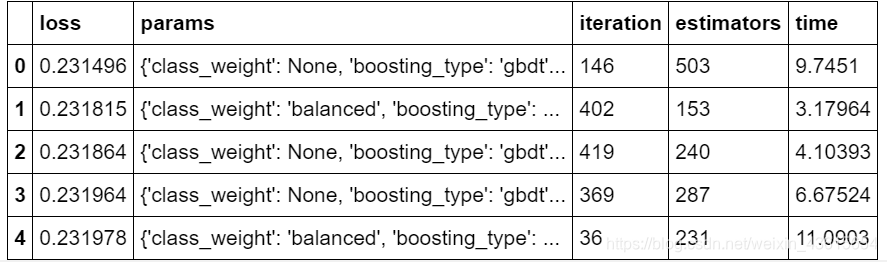
-Random Search Performance

根据运算结果选择参数，用测试集评估它们。
选择最好表现的一组。
因为电脑实在太慢，以下都是抄的我自己没跑……

random_results.loc[0, 'params']

#运行
{'boosting_type': 'gbdt',
 'class_weight': None,
 'colsample_bytree': 0.6444444444444444,
 'learning_rate': 0.006945380919765311,
 'metric': 'auc',
 'min_child_samples': 255,
 'num_leaves': 41,
 'reg_alpha': 0.5918367346938775,
 'reg_lambda': 0.5102040816326531,
 'subsample': 0.803030303030303,
 'subsample_for_bin': 120000,
 'verbose': 1}

用随机搜索的参数训练模型并进行评估

# Find the best parameters and number of estimators
best_random_params = random_results.loc[0, 'params'].copy()
best_random_estimators = int(random_results.loc[0, 'estimators'])
best_random_model = lgb.LGBMClassifier(n_estimators=best_random_estimators, n_jobs = -1, 
                                       objective = 'binary', **best_random_params, random_state = 50)

# Fit on the training data
best_random_model.fit(features, labels)

# Make test predictions
predictions = best_random_model.predict_proba(test_features)[:, 1]


print('The best model from random search scores {:.4f} on the test data.'.format(roc_auc_score(test_labels, predictions)))
print('This was achieved using {} search iterations.'.format(random_results.loc[0, 'iteration']))

结果

The best model from random search scores 0.7232 on the test data.
This was achieved using 146 search iterations.

开始贝叶斯调优

1.目标函数
我们试图最小化目标函数。其输入为一组值——在本例中为 GBM 的超参数，输出为需要最小化的实值——交叉验证损失。Hyperopt 将目标函数作为黑盒处理，因为这个库只关心输入和输出是什么。为了找到使损失最小的输入值，该算法不需要知道目标函数的内部细节！从一个高度抽象的层次上说（以伪代码的形式），我们的目标函数可以表示为：

from hyperopt import STATUS_OK

def objective(params,n_folds = N_FLODS):
    cv_results = lgb.cv(params,train_set,nfold=n_folds,num_boost_round=10000,early_stopping_rounds=100,metrics='auc',seed=50)
    best_score = max(cv_results['auc-mean'])
    loss = 1 - best_score
    return {'loss':loss,'params':params,'status':STATUS_OK}

核心的代码为「cv_results = lgb.cv(…)」。为了实现带早停止的交叉验证，我们使用了 LightGBM 的函数「cv」，向该函数传入的参数包含超参数、一个训练集、交叉验证中使用的许多折，以及一些其它的参数。我们将评估器的数量（num_boost_round）设置为 10000，但是由于我们使用了「early_stopping_rounds」，当 100 个评估器的验证得分没有提高时训练会被停止，所以实际上使用的评估器不会达到这个数量。早停止是一种有效的选择评估器数量的方法，而不是将其设置为另一个需要调优的超参数！

当交叉验证完成后，我们将得到最高得分（ROC AUC）。之后，由于我们想要得到的是最小值，我们将采用「1-最高得分」。该值将在返回的字典数据结构中作为「loss」关键字返回。

这个目标函数实际上比它所需的结构复杂一些，因为我们将返回一个值的字典。对于 Hyperopt 中的目标函数，我们可以返回一个单一的值（即损失），或者返回一个带有最小值的关键字「loss」和「status」的字典。返回超参数的值使我们能够查看每组超参数得到的损失。
2.域空间(domain)
域空间表示我们想要对每个超参数进行评估的值的范围。在每一轮搜索迭代中，贝叶斯优化算法将从域空间中为每个超参数选定一个值。当我们进行随机搜索或网格搜索时，域空间就是一个网格。贝叶斯优化中也是如此，只是这个域空间对每个超参数来说是一个概率分布而不是离散的值。

然而，在贝叶斯优化问题中，确定域空间是最难的部分。如果有机器学习方法的相关经验，我们可以将更大的概率赋予我们认为最佳值可能存在的点，以此来启发对超参数分布的选择。但是，不同的数据集之间的最佳模型设定是不同的，并且具有高维度的问题（大量的超参数），这会使我们很难弄清超参数之间的相互作用。在不确定最佳值的情况下，我们可以使用更大范围的概率分布，通过贝叶斯算法进行推理。

lgb的超参数的值上面写过了这里就不再弄。
虽然我也不想用机翻，但为了不浪费时间就好好用我的复制粘贴大法了：

我不确定世界上是否真有人知道所有的这些超参数是如何相互作用的！而其中有一些超参数是不需要调优（如「objective」和「random_state」）。我们将使用早停止方法找到最佳的评估器数量「n_estimators」。尽管如此，我们仍然需要优化 10 个超参数！当我们第一次对一个模型进行调优时，我通常创建一个以缺省值为中心的大范围域空间，然后在接下来的搜索中对其进行优化。

举个例子，我们不妨在 Hyperopt 中定义一个简单的域——一个离散均匀分布，其中离散点的数量为 GBM 中每棵决策树的叶子结点数：

from hyperopt import hp
from hyperopt.pyll.stochastic import sample
# Discrete uniform distribution
num_leaves = {'num_leaves': hp.quniform('num_leaves', 30, 150, 1)}
num_leaves_dist = []

for _ in range(10000):
    num_leaves_dist.append(sample(num_leaves)['num_leaves'])

plt.figure(figsize=(8,6))
sns.kdeplot(num_leaves_dist,linewidth=2,shade=True)
plt.title('Number of Leaves Distribution',size=18)
plt.title('Number of Leaves Distribution', size = 18)
plt.xlabel('Number of Leaves', size = 16)
plt.ylabel('Density', size = 16)
plt.show()

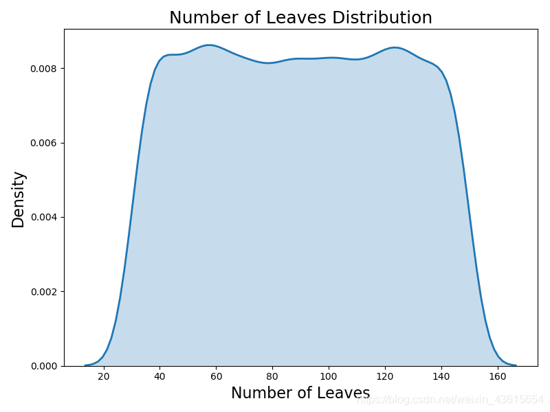
这里使用的是一个离散均匀分布，因为叶子结点的数量必须是一个整数（离散的）并且域中的每个值出现的概率是均等的（均匀）。

概率分布的另一种选项是对数均匀分布，在对数尺度上其值的分布是均匀的。我们将对学习率使用一个对数均匀分布（域空间从 0.005 到 0.2），因为它的值往往在不同的数量级之间变化：

from hyperopt import hp
from hyperopt.pyll.stochastic import sample
# Discrete uniform distribution
num_leaves = {'num_leaves': hp.quniform('num_leaves', 30, 150, 1)}

# Learning rate log uniform distribution
learning_rate = {'learning_rate': hp.loguniform('learning_rate',
                                                 np.log(0.005),
                                                 np.log(0.2))}
learning_rate_dist = []

for i in range(10000):
    learning_rate_dist.append(sample(learning_rate)['learning_rate'])

plt.figure(figsize=(8, 6))
sns.kdeplot(learning_rate_dist, color='red', linewidth=2, shade=True)
plt.title('Learning Rate Distribution', size=18)
plt.xlabel('Learning Rate', size=16)
plt.ylabel('Density', size=16)
plt.show()

-现在开始定义整个域

from hyperopt import hp
from hyperopt.pyll.stochastic import sample
# Define the search space
space = {
    'class_weight': hp.choice('class_weight', [None, 'balanced']),
    'boosting_type': hp.choice('boosting_type', 
                               [{'boosting_type': 'gbdt', 
                                    'subsample': hp.uniform('gdbt_subsample', 0.5, 1)}, 
                                 {'boosting_type': 'dart', 
                                     'subsample': hp.uniform('dart_subsample', 0.5, 1)},
                                 {'boosting_type': 'goss'}]),
    'num_leaves': hp.quniform('num_leaves', 30, 150, 1),
    'learning_rate': hp.loguniform('learning_rate', np.log(0.01), np.log(0.2)),
    'subsample_for_bin': hp.quniform('subsample_for_bin', 20000, 300000, 20000),
    'min_child_samples': hp.quniform('min_child_samples', 20, 500, 5),
    'reg_alpha': hp.uniform('reg_alpha', 0.0, 1.0),
    'reg_lambda': hp.uniform('reg_lambda', 0.0, 1.0),
    'colsample_bytree': hp.uniform('colsample_by_tree', 0.6, 1.0)
}

此处我们使用许多不同种类的域分布：

• choice：类别变量

• quniform：离散均匀分布（在整数空间上均匀分布）

• uniform：连续均匀分布（在浮点数空间上均匀分布）

• loguniform：连续对数均匀分布（在浮点数空间中的对数尺度上均匀分布）

前面提到过，boosting_type的选择会影响到subsample的取值，因此，我们需要使用一个条件域，它意味着一个超参数的值依赖于另一个超参数的值。对于「goss」类型的提升算法，GBM 不能使用下采样技术（选择一个训练观测数据的子样本部分用于每轮迭代）。因此，如果提升的类型为「goss」，则下采样率设置为 1.0（不使用下采样），否则将其设置为 0.5-1.0。这个过程是使用嵌套域实现的。

当我们使用参数完全不同的机器学习模型时，条件嵌套往往是很有用的。条件嵌套让我们能根据「choice」的不同值使用不同的超参数集。

现在已经定义了域空间，我们可以从中提取一个样本来查看典型样本的形式。当我们进行采样时，因为子样本最初是嵌套的，所以我们需要将它分配给顶层的关键字。这个操作是通过 Python 字典的「get」方法实现的，缺省值为 1.0。

# boosting type domain 
boosting_type = {'boosting_type': hp.choice('boosting_type', 
                                            [{'boosting_type': 'gbdt', 'subsample': hp.uniform('subsample', 0.5, 1)}, 
                                             {'boosting_type': 'dart', 'subsample': hp.uniform('subsample', 0.5, 1)},
                                             {'boosting_type': 'goss', 'subsample': 1.0}])}

# Draw a sample
params = sample(boosting_type)
params

从Domain中采样

# Sample from the full space
x = sample(space)

# Conditional logic to assign top-level keys
subsample = x['boosting_type'].get('subsample', 1.0)
x['boosting_type'] = x['boosting_type']['boosting_type']
x['subsample'] = subsample
print(x)

#运行结果1
{'boosting_type': 'goss', 'class_weight': None, 'colsample_bytree': 0.7366231307966129, 'learning_rate': 0.1398679010119344, 'min_child_samples': 380.0, 'num_leaves': 73.0, 'reg_alpha': 0.5266573540445147, 'reg_lambda': 0.889404989776478, 'subsample_for_bin': 20000.0, 'subsample': 1.0}

#再运行一次
{'boosting_type': 'goss', 'class_weight': None, 'colsample_bytree': 0.895519861622759, 'learning_rate': 0.02470781377355416, 'min_child_samples': 50.0, 'num_leaves': 112.0, 'reg_alpha': 0.30733406661439966, 'reg_lambda': 0.4114311595001603, 'subsample_for_bin': 200000.0, 'subsample': 1.0}

-优化算法：

尽管从概念上来说，这是贝叶斯优化最难的一部分，但在 Hyperopt 中创建优化算法只需一行代码。使用树形 Parzen 评估器（Tree Parzen Estimation，以下简称 TPE）的代码如下：

from hyperopt import tpe
# Algorithm
tpe_algorithm = tpe.suggest

这就是优化算法的所有代码！Hyperopt 目前只支持 TPE 和随机搜索，尽管其 GitHub 主页声称将会开发其它方法。在优化过程中，TPE 算法从过去的搜索结果中构建出概率模型，并通过最大化预期提升（EI）来决定下一组目标函数中待评估的超参数。

- 结果历史数据

跟踪这些结果并不是绝对必要的，因为 Hyperopt 会在内部为算法执行此操作。然而，如果我们想要知道这背后发生了什么，我们可以使用「Trials」对象，它将存储基本的训练信息，还可以使用目标函数返回的字典（包含损失「loss」和参数「params」）。创建一个「Trials」对象也仅需一行代码：

from hyperopt import Trials
# Trials object to track progress
bayes_trials = Trials()

作为参考，500 轮随机搜索返回一个在测试集上 ROC AUC 得分为 0.7232、在交叉验证中得分为 0.76850 的模型。一个没有经过优化的缺省模型在测试集上的 ROC AUC 得分则为 0.7143.

当我们查看结果时，需要将以下几点重要事项牢记于心：

最优的超参数在交叉验证中表现最好，但并不一定在测试数据上表现最好。当我们使用交叉验证时，我们希望这些结果能够泛化至测试数据上。

即使使用 10 折交叉验证，超参数调优还是会对训练数据过度拟合。交叉验证取得的最佳得分远远高于在测试数据上的得分。

随机搜索可能由于运气好而返回更好的超参数（重新运行 notebook 就可能改变搜索结果）。贝叶斯优化不能保证找到更好的超参数，并且可能陷入目标函数的局部最小值。

贝叶斯优化虽然十分有效，但它并不能解决我们所有的调优问题。随着搜索的进行，该算法将从探索——尝试新的超参数值，转向开发——利用使目标函数损失最低的 超参数值。如果算法找到了目标函数的一个局部最小值，它可能会专注于搜索局部最小值附近的超参数值，而不会尝试域空间中相对于局部最小值较远的其他值。随机搜索则不会受到这个问题的影响，因为它不会专注于搜索任何值。