利用Shap解释Xgboost（或者别的）模型

Shap的一些介绍：
SHAP包
算法解析
shap的中文解析
知乎的翻译
ps,sklearn库的模型可以用lime模块解析

DEMO1

参（chao)考(xi)利用SHAP解释Xgboost模型
数据集
数据集基本做了特征处理，就基本也不处理别的了。

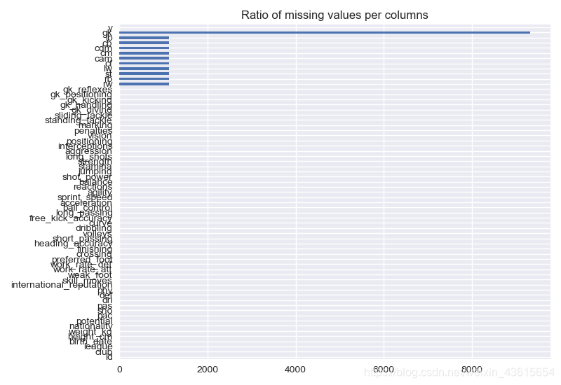
检查下缺失值

print(data.isnull().sum().sort_values(ascending=False))

gk                          9315
cam                         1126
rw                          1126
rb                          1126
st                          1126
cf                          1126
lw                          1126
cm                          1126
cdm                         1126
cb                          1126
lb                          1126

data.isnull().sum(axis=0).plot.barh()
plt.title("Ratio of missing values per columns")
plt.show()

获取年龄

days = today - data['birth_date']
print(days.head())

0    8464 days
1   12860 days
2    7487 days
3   11457 days
4   14369 days
Name: birth_date, dtype: timedelta64[ns]

关于年龄计算这一块

day2 = (today - data['birth_date'])

0    8464 days
1   12860 days
2    7487 days
3   11457 days
4   14369 days
Name: birth_date, dtype: timedelta64[ns]

day2 = (today - data['birth_date']).apply(lambda x: x.days)
#把天数提取成整数

0     8464
1    12860
2     7487
3    11457
4    14369
Name: birth_date, dtype: int64

获得年龄特征

data['age'] = np.round((today - data['birth_date']).apply(lambda x: x.days) / 365., 1)

建立模型和输出

随便选一些特征训练（主要是学习一下shap的用法）

Feature importance：可以直观地反映出特征的重要性，看出哪些特征对最终的模型影响较大。但是无法判断特征与最终预测结果的关系是如何的。

cols = ['height_cm', 'potential', 'pac', 'sho', 'pas', 'dri', 'def', 'phy', 'international_reputation', 'age']

model = xgb.XGBRegressor(max_depth=4, learning_rate=0.05, n_estimators=150)
model.fit(data[cols], data['y'].values)

plt.figure(figsize=(15, 5))
plt.bar(range(len(cols)), model.feature_importances_)
plt.xticks(range(len(cols)), cols, rotation=-45, fontsize=14)
plt.title('Feature importance', fontsize=14)
plt.show()

采用shap（SHapley Additive exPlanation）验证模型

解释器explainer

explainer = shap.TreeExplainer(model)

获取训练集data各个样本各个特征的SHAP值

因为data中有10441个样本以及10个特征，得到的shap_values的维度是10441×10。

shap_values = explainer.shap_values(data[cols])
print(shap_values.shape)

这里我是报错的。没找到原因。应该是自带的BUG。

AssertionError: Additivity check failed in TreeExplainer! Please report this on GitHub. Consider retrying with the feature_dependence='independent' option.

计算基线

y_base = explainer.expected_value
print(y_base)

data['pred'] = model.predict(X_train)
print(data['pred'].mean())

229.16510445903987
229.16512

DEMO2

Explain Your Model with the SHAP Values
Explain Any Models with the SHAP Values — Use the KernelExplainer

导入库

import xgboost as xgb
import pandas as pd
import numpy as np
import matplotlib.pyplot as plt
import seaborn as sns
plt.style.use('seaborn')
pd.set_option('display.max_columns', 1000)
pd.set_option('display.width', 1000)
pd.set_option('display.max_colwidth', 1000)

data = pd.read_csv("C:\\Users\\Nihil\\Documents\\pythonlearn\\data\\kaggle\\winequality-red.csv")

检查数据

print(data.info())

Data columns (total 12 columns):
fixed acidity           1599 non-null float64
volatile acidity        1599 non-null float64
citric acid             1599 non-null float64
residual sugar          1599 non-null float64
chlorides               1599 non-null float64
free sulfur dioxide     1599 non-null float64
total sulfur dioxide    1599 non-null float64
density                 1599 non-null float64
pH                      1599 non-null float64
sulphates               1599 non-null float64
alcohol                 1599 non-null float64
quality                 1599 non-null int64
dtypes: float64(11), int64(1)
memory usage: 150.0 KB
None

print(data.head())

      fixed acidity  volatile acidity  citric acid  residual sugar  chlorides  free sulfur dioxide  total sulfur dioxide  density    pH  sulphates  alcohol  quality
0            7.4              0.70         0.00             1.9      0.076                 11.0                  34.0   0.9978  3.51       0.56      9.4        5
1            7.8              0.88         0.00             2.6      0.098                 25.0                  67.0   0.9968  3.20       0.68      9.8        5
2            7.8              0.76         0.04             2.3      0.092                 15.0                  54.0   0.9970  3.26       0.65      9.8        5
3           11.2              0.28         0.56             1.9      0.075                 17.0                  60.0   0.9980  3.16       0.58      9.8        6
4            7.4              0.70         0.00             1.9      0.076                 11.0                  34.0   0.9978  3.51       0.56      9.4        5

设置feature和target

target = 'quality' 
X_columns = [x for x in data.columns if x not in [target]]
X = data[X_columns]
Y = data['quality']

训练一个随机森林模型

X_train,X_test,y_train,y_test = train_test_split(X,y,test_size=0.3)
model = RandomForestRegressor(max_depth=6, random_state=0, n_estimators=10)
model.fit(X_train, y_train)

（A）Variable Importance Plot — Global Interpretability（全局可解释性）

• 目的：variable importance plot 列出了最重要的变量，顶部特征对预测能力的贡献最大。

import shap
shap_values = shap.TreeExplainer(model).shap_values(X_train)
shap.summary_plot(shap_values, X_train, plot_type="bar")

卧槽跟度数关于这么大么？（重点错

SHAP value plot

• 目的：The SHAP value plot可以进一步显示预测因子与目标变量之间的正、负关系

shap.summary_plot(shap_values, X_train)

图还是很好看的。这个图是由所有训练数据构成，表达以下信息：

• Feature importance 可以看出各特征对预测能力的贡献程度
• Impact: 水平位置显示该值的影响是与较高还是较低的预测相关联。比如图上酒精就与1.0更相关
• Original value 颜色显示该变量是该观察值的高（红色）还是低（蓝色）。
• Correlation 酒精含量高对产品的质量等级有高而积极的影响。高来自红色，positive impact显示在x轴上。同样，挥发性酸度与目标变量呈负相关。

(B) SHAP Dependence Plot — Global Interpretability

含义：部分相关图显示了一个或两个特征对机器学习模型预测结果的边际效应(J. H. Friedman 2001)。
Greedy function approximation: A gradient boosting machine.（上面那篇论文）
Marginal effects measure the expected instantaneous change in the dependent variable as a function of a change in a certain explanatory variable while keeping all the other covariates constant. The marginal effect measurement is required to interpret the effect of the regressors on the dependent variable.
它告诉我们目标和特征之间的关系是线性的、单调的还是更复杂的。
代码如下：

shap.dependence_plot('alcohol',shap_values, X_train)

下图显示“酒精”和目标变量之间存在近似线性和正相关，并且“酒精”经常与“Sulphates”相互作用。

显示关于“挥发性酸度”的Dependence Plot

shap.dependence_plot('volatile acidity',shap_values, X_train)

这是个负相关

© Individual SHAP Value Plot — Local Interpretability（单个特征，局部解释性）

这个图得用Jupyter，我先跳过吧。

X_output = X_test.copy()
X_output.loc[:,'predict'] = np.round(model.predict(X_output),2)
random_picks = np.arange(1,330,50)#随便选点来观察
S = X_output.iloc[random_picks]
print(S)

         fixed acidity  volatile acidity  citric acid  residual sugar  chlorides  free sulfur dioxide  total sulfur dioxide  density    pH  sulphates  alcohol  predict
1146            7.8             0.500         0.12             1.8      0.178                  6.0                  21.0  0.99600  3.28       0.87      9.8     5.51
854             9.3             0.360         0.39             1.5      0.080                 41.0                  55.0  0.99652  3.47       0.73     10.9     5.94
1070            9.3             0.330         0.45             1.5      0.057                 19.0                  37.0  0.99498  3.18       0.89     11.1     6.47
697             7.0             0.650         0.02             2.1      0.066                  8.0                  25.0  0.99720  3.47       0.67      9.5     5.39
1155            8.3             0.600         0.25             2.2      0.118                  9.0                  38.0  0.99616  3.15       0.53      9.8     5.17
1553            7.3             0.735         0.00             2.2      0.080                 18.0                  28.0  0.99765  3.41       0.60      9.4     5.24
99              8.1             0.545         0.18             1.9      0.080                 13.0                  35.0  0.99720  3.30       0.59      9.0     5.27

对多个变量的交互进行分析

shap_interaction_values = shap.TreeExplainer(model).shap_interaction_values(X_train)
shap.summary_plot(shap_interaction_values, X_train, max_display=4)