二维图像的功率谱分析与计算

原理：
对于MxN的数字图像f(x,y),其二维傅里叶变换的公式为：

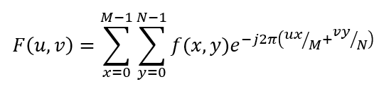
u和v分别在0，1，…,M-1和0，1，…,N-1取值。

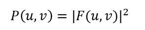
而功率谱的定义为：

1. matlab代码实现：

clc; clear all; close all;
img = imread('a.jpg','jpg');
img = rgb2gray(img);    
% 图像的功率谱
psd = abs(fftshift(fft2(img))).^2
% 通过对数变换，便于观察
psd = 10 * log10(psd); 
mesh(psd)

2. python代码实现（批处理，求数据集的平均功率谱）

from PIL import Image
from numpy.fft import fft2, fftshift
import matplotlib.pyplot as plt
import numpy as np

def calculate_psd(imgPath):
	srcIm = Image.open(imgPath).convert('L')
	# 图像的功率谱
	fd_Im = fftshift(fft2(srcIm))
	psd = abs(fd_Im) ** 2
	# psd = 10 * np.log10(psd)
	return psd

## power spectral
path = r'D:\Project\edges2shoes\results\edges2shoes'
label = '_generated'
fpath_list = []
for root, _, fnames in sorted(os.walk(path, followlinks=True)):
	for fname in fnames:
		if label in fname:
			fpath_list.append(os.path.join(root, fname))

average_psd = []
for i in range(len(fpath_list)):
	psd = calculate_psd(fpath_list[i])
	average_psd.append(psd)
average_psd = sum(average_psd) / len(fpath_list)
# 通过对数变换，便于观察
average_psd = 10 * np.log10(average_psd)

# Plot the surface.
fig = plt.figure()
ax = fig.gca(projection='3d')
X = np.arange(0, 256)
Y = np.arange(0, 256)
X, Y = np.meshgrid(X, Y)
surf = ax.plot_surface(X, Y, average_psd)
# Add a color bar which maps values to colors.
fig.colorbar(surf, shrink=0.5, aspect=5)
plt.show()
plt.savefig("gt_py.png")