XGBoost实战

1.XGBoost介绍

• 简介：XGBoost是boosting算法的其中一种。Boosting算法的思想是将许多弱分类器集成在一起形成一个强分类器。因为XGBoost是一种提升树模型，所以它是将许多树模型集成在一起，形成一个很强的分类器。而所用到的树模型则是CART回归树模型。

• 算法思想：该算法思想就是不断地添加树，不断地进行特征分裂来生长一棵树，每次添加一个树，其实是学习一个新函数，去拟合上次预测的残差。当我们训练完成得到k棵树，我们要预测一个样本的分数，其实就是根据这个样本的特征，在每棵树中会落到对应的一个叶子节点，每个叶子节点就对应一个分数，最后只需要将每棵树对应的分数加起来就是该样本的预测值。

• 过拟合：
  XGBoost还提出了两种防止过拟合的方法：Shrinkage and Column Subsampling。Shrinkage方法就是在每次迭代中对树的每个叶子结点的分数乘上一个缩减权重η，这可以使得每一棵树的影响力不会太大，留下更大的空间给后面生成的树去优化模型。Column Subsampling类似于随机森林中的选取部分特征进行建树。其可分为两种，一种是按层随机采样，在对同一层内每个结点分裂之前，先随机选择一部分特征，然后只需要遍历这部分的特征，来确定最优的分割点。另一种是随机选择特征，则建树前随机选择一部分特征然后分裂就只遍历这些特征。一般情况下前者效果更好。

  可以设置树的最大深度、当样本权重和小于设定阈值时停止生长去防止过拟合

• XGBoost的优点
  之所以XGBoost可以成为机器学习的大杀器，广泛用于数据科学竞赛和工业界，是因为它有许多优点：
  1.使用许多策略去防止过拟合，如：正则化项、Shrinkage and Column Subsampling等。
  2.目标函数优化利用了损失函数关于待求函数的二阶导数
  3.支持并行化，这是XGBoost的闪光点，虽然树与树之间是串行关系，但是同层级节点可并行。具体的对于某个节点，节点内选择最佳分裂点，候选分裂点计算增益用多线程并行。训练速度快。
  4.添加了对稀疏数据的处理。
  5.交叉验证，early stop，当预测结果已经很好的时候可以提前停止建树，加快训练速度。
  6.支持设置样本权重，该权重体现在一阶导数g和二阶导数h，通过调整权重可以去更加关注一些样本。

• GB、GBDT、xgboost的理解 https://www.cnblogs.com/wxquare/p/5541414.html

2.数据展示

2.1 查看形状

import pandas as pd
import numpy as np
import matplotlib.pyplot as plt
from sklearn.linear_model import LogisticRegression
from sklearn.ensemble import RandomForestClassifier
from sklearn.metrics import roc_auc_score as AUC
from sklearn.metrics import mean_absolute_error
from sklearn.decomposition import PCA
from sklearn.preprocessing import LabelEncoder, LabelBinarizer
from sklearn.model_selection import cross_val_score

from scipy import stats
import seaborn as sns
from copy import deepcopy
train = pd.read_csv('train.csv')
test = pd.read_csv('test.csv')
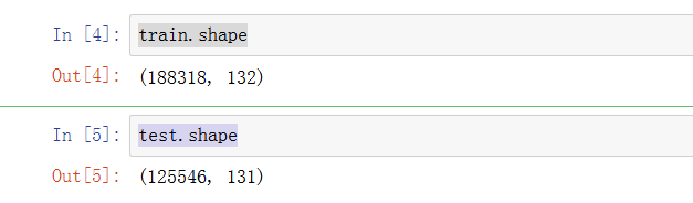
train.shape
test.shape

2.2 查看列和描述信息

print ('First 20 columns:', list(train.columns[:20]))
print ('Last 20 columns:', list(train.columns[-20:]))

我们看到，大概有116个种类属性（如它们的名字所示）和14个连续（数字）属性。 此外，还有ID和赔偿。总计为132列。

train.describe()

正如我们看到的，所有的连续的功能已被缩放到[0,1]区间，均值基本为0.5。其实数据已经被预处理了，我们拿到的是特征数据。

2.3 查看缺失值

pd.isnull(train).values.any()

没有缺失值

2.4 查看数据集的信息

train.info()

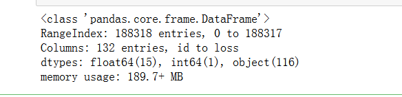
在这里，float64(15)、int 64(1)是我们的连续特征（带有int 64的可能是ID），而对象(116)是分类特征。

• 查看object属性的列数

cat_features = list(train.select_dtypes(include=['object']).columns)
print(len(cat_features))

• 查看float64,int64属性的列数

cont_features = [cont for cont in list(train.select_dtypes(
                 include=['float64', 'int64']).columns) if cont not in ['loss', 'id']]
print(len(cont_features))
print(cont_features)

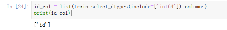
• 查看int64t属性的列数
  

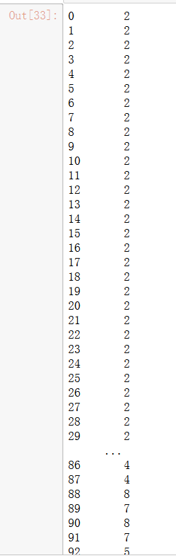
2.5 类别值中属性的个数

cat_uniques = []
for cat in cat_features:
    cat_uniques.append(len(train[cat].unique())) 
uniq_values_in_categories = pd.DataFrame.from_items([('cat_name', cat_features), ('unique_values', cat_uniques)])
uniq_values_in_categories.head()
uniq_values_in_categories.unique_values

• 类别值中属性的个数绘图

fig, (ax1, ax2) = plt.subplots(1,2)
fig.set_size_inches(16,5)
ax1.hist(uniq_values_in_categories.unique_values, bins=50)
ax1.set_title('Amount of categorical features with X distinct values')
ax1.set_xlabel('Distinct values in a feature')
ax1.set_ylabel('Features')
ax1.annotate('A feature with 326 vals', xy=(322, 2), xytext=(200, 38), arrowprops=dict(facecolor='black'))

ax2.set_xlim(2,30)
ax2.set_title('Zooming in the [0,30] part of left histogram')
ax2.set_xlabel('Distinct values in a feature')
ax2.set_ylabel('Features')
ax2.grid(True)
ax2.hist(uniq_values_in_categories[uniq_values_in_categories.unique_values <= 30].unique_values, bins=30)
ax2.annotate('Binary features', xy=(3, 71), xytext=(7, 71), arrowprops=dict(facecolor='black'))

正如我们所看到的，大部分的分类特征（72/116）是二值的，绝大多数特征（88/116）有四个值，其中有一个具有326个值的特征（一天的数量）。

2.6 赔偿值

print(len(train['id']))
plt.figure(figsize=(16,8))
plt.plot(train['id'], train['loss'])
plt.title('Loss values per id')
plt.xlabel('id')
plt.ylabel('loss')
plt.legend()
plt.show()

损失值中有几个显著的峰值表示严重事故。这样的数据分布，使得这个功能非常扭曲导致的回归表现不佳。
基本上，偏度度量了实值随机变量的均值分布的不对称性。

• 计算损失的偏度：

stats.mstats.skew(train['loss'])#计算数据集的偏度

数据确实是倾斜的
对数据进行对数变换通常可以

• 改善倾斜，使用 np.log

stats.mstats.skew(np.log(train['loss'])).data

• 损失值绘制直方图对比

fig, (ax1, ax2) = plt.subplots(1,2)
fig.set_size_inches(16,5)
ax1.hist(train['loss'], bins=50)
ax1.set_title('Train Loss target histogram')
ax1.grid(True)
ax2.hist(np.log(train['loss']), bins=50, color='g')
ax2.set_title('Train Log Loss target histogram')
ax2.grid(True)
plt.show()

2.7 连续值特征

• 绘制数值特征的直方图并分析它们的分布：

train[cont_features].hist(bins=50, figsize=(16,12))

2.8 特征之间的相关性

plt.subplots(figsize=(16,9))
correlation_mat = train[cont_features].corr()
sns.heatmap(correlation_mat, annot=True)

3. XGBoost基本模型构建过程

import xgboost as xgb
import pandas as pd
import numpy as np
import pickle
import sys
import matplotlib.pyplot as plt
from sklearn.metrics import mean_absolute_error, make_scorer
from sklearn.preprocessing import StandardScaler
from sklearn.model_selection import GridSearchCV
from scipy.sparse import csr_matrix, hstack
from sklearn.cross_validation import KFold, train_test_split
from xgboost import XGBRegressor

import warnings
warnings.filterwarnings('ignore')

3.1 数据预处理

• 做对数转换

train = pd.read_csv('train.csv')
train['log_loss'] = np.log(train['loss'])
features = [x for x in train.columns if x not in ['id','loss', 'log_loss']]

cat_features = [x for x in train.select_dtypes(
        include=['object']).columns if x not in ['id','loss', 'log_loss']]
num_features = [x for x in train.select_dtypes(
        exclude=['object']).columns if x not in ['id','loss', 'log_loss']]

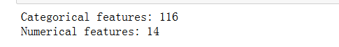
print ("Categorical features:", len(cat_features))
print ("Numerical features:", len(num_features))

• 数据分成连续和离散特征
  
• 对分类特性使用标签编码器

ntrain = train.shape[0]

train_x = train[features]
train_y = train['log_loss']

for c in range(len(cat_features)):
    train_x[cat_features[c]] = train_x[cat_features[c]].astype('category').cat.codes
    
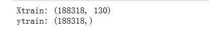
print ("Xtrain:", train_x.shape)
print ("ytrain:", train_y.shape)

3.2 使用 xgb.DMatrix对数据预处理

首先，我们训练一个基本的xgboost模型，然后进行参数调节通过交叉验证来观察结果的变换，使用平均绝对误差来衡量
mean_absolute_error(np.exp(y), np.exp(yhat))。
xgboost 自定义了一个数据矩阵类 DMatrix，会在训练开始时进行一遍预处理，从而提高之后每次迭代的效率

def xg_eval_mae(yhat, dtrain):
    y = dtrain.get_label()
    return 'mae', mean_absolute_error(np.exp(y), np.exp(yhat))

Model

dtrain = xgb.DMatrix(train_x, train['log_loss'])

Xgboost参数

• ‘booster’:‘gbtree’,
• ‘objective’: ‘multi:softmax’, 多分类的问题
• ‘num_class’:10, 类别数，与 multisoftmax 并用
• ‘gamma’:损失下降多少才进行分裂
• ‘max_depth’:12, 构建树的深度，越大越容易过拟合
• ‘lambda’:2, 控制模型复杂度的权重值的L2正则化项参数，参数越大，模型越不容易过拟合。
• ‘subsample’:0.7, 随机采样训练样本
• ‘colsample_bytree’:0.7, 生成树时进行的列采样
• ‘min_child_weight’:3, 孩子节点中最小的样本权重和。如果一个叶子节点的样本权重和小于min_child_weight则拆分过程结束
• ‘silent’:0 ,设置成1则没有运行信息输出，最好是设置为0.
• ‘eta’: 0.007, 如同学习率
• ‘seed’:1000,
• ‘nthread’:7, cpu 线程数

3.3 xgb_params

xgb_params = {
    'seed': 0,
    'eta': 0.1,
    'colsample_bytree': 0.5,
    'silent': 1,
    'subsample': 0.5,
    'objective': 'reg:linear',
    'max_depth': 5,
    'min_child_weight': 3
}

3.4 使用交叉验证 xgb.cv

bst_cv1 = xgb.cv(xgb_params, dtrain, num_boost_round=50, nfold=3, seed=0, 
                feval=xg_eval_mae, maximize=False, early_stopping_rounds=10)
print ('CV score:', bst_cv1.iloc[-1,:]['test-mae-mean'])

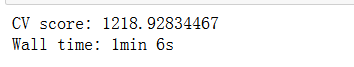
我们得到了第一个基准结果：MAE＝1218.9

3.5 绘制训练和测试的平均绝对误差变化图

plt.figure()
bst_cv1[['train-mae-mean', 'test-mae-mean']].plot()

我们的第一个基础模型：，没有发生过拟合，只建立了50个树模型

3.6 建立100个树模型的变化

bst_cv2 = xgb.cv(xgb_params, dtrain, num_boost_round=100, 
                nfold=3, seed=0, feval=xg_eval_mae, maximize=False, 
                early_stopping_rounds=10)

print ('CV score:', bst_cv2.iloc[-1,:]['test-mae-mean'])

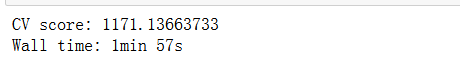
可以观察到，模型效果更好，训练时间也更长

• 绘制100个树模型训练和测试的平均绝对误差变化图

fig, (ax1, ax2) = plt.subplots(1,2)
fig.set_size_inches(16,4)

ax1.set_title('100 rounds of training')
ax1.set_xlabel('Rounds')
ax1.set_ylabel('Loss')
ax1.grid(True)
ax1.plot(bst_cv2[['train-mae-mean', 'test-mae-mean']])
ax1.legend(['Training Loss', 'Test Loss'])

ax2.set_title('60 last rounds of training')
ax2.set_xlabel('Rounds')
ax2.set_ylabel('Loss')
ax2.grid(True)
ax2.plot(bst_cv2.iloc[40:][['train-mae-mean', 'test-mae-mean']])
ax2.legend(['Training Loss', 'Test Loss'])

有那么一丁丁过拟合，现在还没多大事
我们得到了新的纪录 MAE = 1171.77 比第一次的要好 (1218.9). 接下来我们要改变其他参数了。

4.XGBoost 参数调节过程

4.1 调节的参数

• Step 1: 选择一组初始参数
• Step 2: 改变 max_depth 和 min_child_weight.
• Step 3: 调节 gamma 降低模型过拟合风险.
• Step 4: 调节 subsample 和 colsample_bytree 改变数据采样策略.
• Step 5: 调节学习率 eta.

将XGBoostRegressor封装成类

class XGBoostRegressor(object):
    def __init__(self, **kwargs):
        self.params = kwargs
        if 'num_boost_round' in self.params:
            self.num_boost_round = self.params['num_boost_round']
        self.params.update({'silent': 1, 'objective': 'reg:linear', 'seed': 0})
        
    def fit(self, x_train, y_train):
        dtrain = xgb.DMatrix(x_train, y_train)
        self.bst = xgb.train(params=self.params, dtrain=dtrain, num_boost_round=self.num_boost_round,
                             feval=xg_eval_mae, maximize=False)
        
    def predict(self, x_pred):
        dpred = xgb.DMatrix(x_pred)
        return self.bst.predict(dpred)
    
    def kfold(self, x_train, y_train, nfold=5):
        dtrain = xgb.DMatrix(x_train, y_train)
        cv_rounds = xgb.cv(params=self.params, dtrain=dtrain, num_boost_round=self.num_boost_round,
                           nfold=nfold, feval=xg_eval_mae, maximize=False, early_stopping_rounds=10)
        return cv_rounds.iloc[-1,:]
    
    def plot_feature_importances(self):
        feat_imp = pd.Series(self.bst.get_fscore()).sort_values(ascending=False)
        feat_imp.plot(title='Feature Importances')
        plt.ylabel('Feature Importance Score')
        
    def get_params(self, deep=True):
        return self.params
 
    def set_params(self, **params):
        self.params.update(params)
        return self

• mae_score取平均绝对误差

def mae_score(y_true, y_pred):
    return mean_absolute_error(np.exp(y_true), np.exp(y_pred))
mae_scorer = make_scorer(mae_score, greater_is_better=False)

bst = XGBoostRegressor(eta=0.1, colsample_bytree=0.5, subsample=0.5, 
                       max_depth=5, min_child_weight=3, num_boost_round=50)
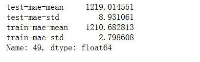
bst.kfold(train_x, train_y, nfold=5)

交叉验证后的值：

4.2 Step 1: 基准模型

4.3 Step 2: 树的深度与节点权重

这些参数对xgboost性能影响最大，因此，他们应该调整第一。
我们简要地概述它们：

• max_depth: 树的最大深度。增加这个值会使模型更加复杂，也容易出现过拟合，深度3-10是合理的。
• min_child_weight: 正则化参数. 如果树分区中的实例权重小于定义的总和，则停止树构建过程。

xgb_param_grid = {'max_depth': list(range(4,9)), 'min_child_weight': list((1,3,6))}
xgb_param_grid['max_depth']

• 使用GridSearchCV()函数设置参数
  它存在的意义就是自动调参，只要把参数输进去，就能给出最优化的结果和参数。但是这个方法适合于小数据集，一旦数据的量级上去了，很难得出结果。

grid = GridSearchCV(XGBoostRegressor(eta=0.1, num_boost_round=50, colsample_bytree=0.5, subsample=0.5),
                param_grid=xgb_param_grid, cv=5, scoring=mae_scorer)

• 训练模型

grid.fit(train_x, train_y.values)

• 打印评分

grid.grid_scores_, grid.best_params_, grid.best_score_

网格搜索发现的最佳结果:
{‘max_depth’: 8, ‘min_child_weight’: 6}, -1187.9597499123447)
设置成负的值是因为要找大的值

• 绘制模型使用交叉验证的随min_child_weight，max_depth的值而变化图

def convert_grid_scores(scores):
    _params = []
    _params_mae = []    
    for i in scores:
        _params.append(i[0].values())
        _params_mae.append(i[1])
    params = np.array(_params)
    grid_res = np.column_stack((_params,_params_mae))
    return [grid_res[:,i] for i in range(grid_res.shape[1])]
_,scores =  convert_grid_scores(grid.grid_scores_)
scores = scores.reshape(5,3)

plt.figure(figsize=(10,5))
cp = plt.contourf(xgb_param_grid['min_child_weight'], xgb_param_grid['max_depth'], scores, cmap='BrBG')
plt.colorbar(cp)
plt.title('Depth / min_child_weight optimization')
plt.annotate('We use this', xy=(5.95, 7.95), xytext=(4, 7.5), arrowprops=dict(facecolor='white'), color='white')
plt.annotate('Good for depth=7', xy=(5.98, 7.05), 
             xytext=(4, 6.5), arrowprops=dict(facecolor='white'), color='white')
plt.xlabel('min_child_weight')
plt.ylabel('max_depth')
plt.grid(True)
plt.show()

我们看到，从网格搜索的结果，分数的提高主要是基于max_depth增加. min_child_weight稍有影响的成绩，但是，我们看到，min_child_weight = 6会更好一些。

4.4 Step 3: 调节 gamma去降低过拟合风险

• 调节参数

xgb_param_grid = {'gamma':[ 0.1 * i for i in range(0,5)]}

grid = GridSearchCV(XGBoostRegressor(eta=0.1, num_boost_round=50, max_depth=8, min_child_weight=6,
                                        colsample_bytree=0.5, subsample=0.5),
                    param_grid=xgb_param_grid, cv=5, scoring=mae_scorer)
grid.fit(train_x, train_y.values)

• 打印均值

grid.grid_scores_, grid.best_params_, grid.best_score_

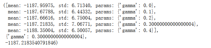
差别并不大，我们选择使用偏小一些的 gamma

4.5 Step 4: 调节样本采样方式 subsample 和 colsample_bytree

xgb_param_grid = {'subsample':[ 0.1 * i for i in range(6,9)],
                      'colsample_bytree':[ 0.1 * i for i in range(6,9)]}


grid = GridSearchCV(XGBoostRegressor(eta=0.1, gamma=0.2, num_boost_round=50, max_depth=8, min_child_weight=6),
                    param_grid=xgb_param_grid, cv=5, scoring=mae_scorer)
grid.fit(train_x, train_y.values)

grid.grid_scores_, grid.best_params_, grid.best_score_

• 绘制调节subsample 和 colsample_bytree参数过程中分值的变化图

_, scores =  convert_grid_scores(grid.grid_scores_)
scores = scores.reshape(3,3)

plt.figure(figsize=(10,5))
cp = plt.contourf(xgb_param_grid['subsample'], xgb_param_grid['colsample_bytree'], scores, cmap='BrBG')
plt.colorbar(cp)
plt.title('Subsampling params tuning')
plt.annotate('Optimum', xy=(0.895, 0.6), xytext=(0.8, 0.695), arrowprops=dict(facecolor='black'))
plt.xlabel('subsample')
plt.ylabel('colsample_bytree')
plt.grid(True)
plt.show()

可以明显的看出，最优的参数：‘colsample_bytree’: 0.8, ‘subsample’: 0.8

4.6 Step 5: 减小学习率并增大树个数

参数优化的最后一步是降低学习速度，同时增加更多的估计量

• 调节eta参数：

xgb_param_grid = {'eta':[0.5,0.4,0.3,0.2,0.1,0.075,0.05,0.04,0.03]}
grid = GridSearchCV(XGBoostRegressor(num_boost_round=50, gamma=0.2, max_depth=8, min_child_weight=6,
                                        colsample_bytree=0.6, subsample=0.9),
                    param_grid=xgb_param_grid, cv=5, scoring=mae_scorer)

grid.fit(train_x, train_y.values)

grid.grid_scores_, grid.best_params_, grid.best_score_

• 绘制调节 eta 参数过程中分值的变化图

eta, y = convert_grid_scores(grid.grid_scores_)
plt.figure(figsize=(10,4))
plt.title('MAE and ETA, 50 trees')
plt.xlabel('eta')
plt.ylabel('score')
plt.plot(eta, -y)
plt.grid(True)
plt.show()

{‘eta’: 0.2}, -1160.9736284869114 ,num_boost_round=50 是目前最好的结果

• 把树的个数增加到100

xgb_param_grid = {'eta':[0.5,0.4,0.3,0.2,0.1,0.075,0.05,0.04,0.03]}
grid = GridSearchCV(XGBoostRegressor(num_boost_round=100, gamma=0.2, max_depth=8, min_child_weight=6,
                                        colsample_bytree=0.6, subsample=0.9),
                    param_grid=xgb_param_grid, cv=5, scoring=mae_scorer)

grid.fit(train_x, train_y.values)

grid.grid_scores_, grid.best_params_, grid.best_score_

• 绘制参数为100个树过程中随eta的值变化的分值的变化图

eta, y = convert_grid_scores(grid.grid_scores_)
plt.figure(figsize=(10,4))
plt.title('MAE and ETA, 100 trees')
plt.xlabel('eta')
plt.ylabel('score')
plt.plot(eta, -y)
plt.grid(True)
plt.show()

’eta’: 0.1， -1152.2471498726127，学习率低一些的效果更好

• 200个树呢？

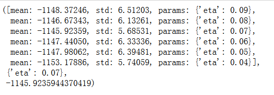
xgb_param_grid = {'eta':[0.09,0.08,0.07,0.06,0.05,0.04]}
grid = GridSearchCV(XGBoostRegressor(num_boost_round=200, gamma=0.2, max_depth=8, min_child_weight=6,
                                        colsample_bytree=0.6, subsample=0.9),
                    param_grid=xgb_param_grid, cv=5, scoring=mae_scorer)
grid.fit(train_x, train_y.values)

• 打印均值值：

grid.grid_scores_, grid.best_params_, grid.best_score_

• 画图

eta, y = convert_grid_scores(grid.grid_scores_)
plt.figure(figsize=(10,4))
plt.title('MAE and ETA, 200 trees')
plt.xlabel('eta')
plt.ylabel('score')
plt.plot(eta, -y)
plt.grid(True)
plt.show()

可以看出，目前在200个树中eta为0.07 mean值最大为-1145.9235944370419

4.7 最优模型

bst = XGBoostRegressor(num_boost_round=200, eta=0.07, gamma=0.2, max_depth=8, min_child_weight=6,
                                        colsample_bytree=0.6, subsample=0.9)
cv = bst.kfold(train_x, train_y, nfold=5)

我们看到200棵树最好的ETA是0.07。正如我们所预料的那样，ETA和num_boost_round依赖关系不是线性的，但是有些关联。
我们花了相当长的一段时间优化xgboost. 从初始值: 1219.57. 经过调参之后达到 MAE=1171.77.
我们还发现参数之间的关系ETA和num_boost_round：

• 100 trees, eta=0.1: MAE=1152.247
• 200 trees, eta=0.07: MAE=1145.92

XGBoostRegressor(num_boost_round=200, gamma=0.2, max_depth=8, min_child_weight=6, colsample_bytree=0.6, subsample=0.9, eta=0.07).

4.8 总结

我们可以清楚地看出，XGBoost模型调参数对模型的上限影响并不是很大，算法和参数的调优只是逼近这一个上限，我们要在数据和特征方面上下文章！