Python气象绘图笔记——常用气象绘图函数脚本封装与使用记录

由于工作需要，将对我常用的python绘图脚本进行封装，为了防止代码丢失、忘记使用流程等，写个博客记录下。
要加载的包

import os
import matplotlib.ticker as mticker
import netCDF4 as nc
import matplotlib.path as mpath
import cmaps
import matplotlib.pyplot as plt###引入库包
import cartopy.mpl.ticker as cticker
import numpy as np
import numpy.ma as ma
import matplotlib as mpl
import cartopy.crs as ccrs
import cartopy.feature as cfeature
from netCDF4 import Dataset
try:
    import pykdtree.kdtree
    _IS_PYKDTREE = True
except ImportError:
    import scipy.spatial
    _IS_PYKDTREE = False
from wrf import getvar, interplevel, vertcross,vinterp, ALL_TIMES, CoordPair, xy_to_ll, ll_to_xy, to_np, get_cartopy, latlon_coords, cartopy_xlim, cartopy_ylim
from cartopy.mpl.gridliner import LONGITUDE_FORMATTER, LATITUDE_FORMATTER
import xarray as xr
import pandas as pd
import datetime as dt
import time

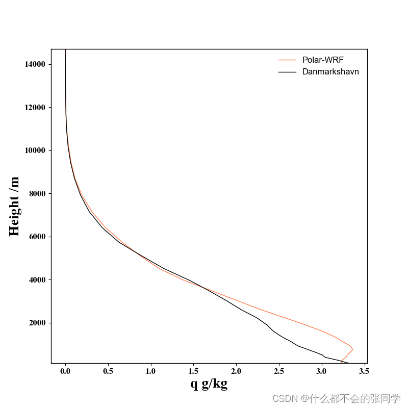
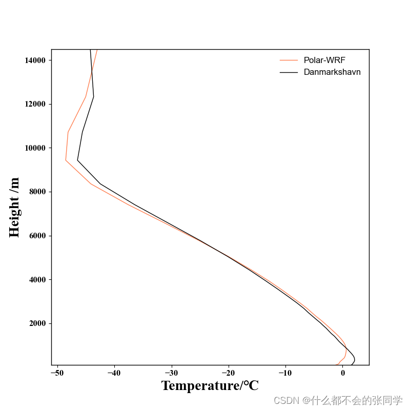
垂直廓线图

垂直廓线图（Profile），指各气象要素在垂直高度上的分布，垂直廓线一般可以用来判断大气垂直结构、层结属性，获取中高层大气的各要素特征。
本文绘制目的：将怀俄明大学探空站点数据与WRF模拟绘制，判断WRF模拟能力。
数据处理：

#WRF变量读取
def nearest_position( stn_lat, stn_lon, xlat, xlon ):
    """获取最临近格点坐标索引
    parameters:
    ----------------------
    lon  : 单个站点经度
    lat  : 单个站点纬度
    lons : numpy.ndarray网格二维经度坐标
    lats : numpy.ndarray网格二维纬度坐标 
    Return:
    -----------------------
    (xindx,yindx)

    """
    difflat = stn_lat - xlat;
    difflon = stn_lon - xlon;
    rad = np.multiply(difflat,difflat)+np.multiply(difflon , difflon)#difflat * difflat + difflon * difflon
    aa=np.where(rad==np.min(rad))
    ind=np.squeeze(np.array(aa))
    return tuple(ind)
stlat=[71.3,72.6,76.8,80.6,76.0,82.5,79.9]
stlon=[-156.8,-38.4,-18.7,58.1,137.9,-62.3,-85.9]
jsta=np.zeros(len(stlat))
ista=np.zeros(len(stlon))
for i in range(0,len(stlat)):
    indexSta = nearest_position(stlat[i], stlon[i], lat2d, lon2d)
    jsta[i]=indexSta[0]
    ista[i]=indexSta[1]

n=int(6)
tk_st=to_np(tk[:,int(jsta[n]),int(ista[n])])
z_st=az[:,int(jsta[n]),int(ista[n])]
q_st=q[:,int(jsta[n]),int(ista[n])]
q_st=to_np(q_st)*1000
wdir_st=to_np(wdir[:,:,int(jsta[n]),int(ista[n])])
wdir_st=np.transpose(wdir_st)
z_st=to_np(z_st)
z_st=z_st
ht=z_st[np.where(z_st<15001)]
q_st=q_st[np.where(z_st<15001)]
tk_st=tk_st[np.where(z_st<15001)]-273.3
wdir_st=wdir_st[np.where(z_st<15001),:]
wrf_data=np.vstack((tk_st,q_st,wdir_st[0,:,1],wdir_st[0,:,0]))
wrf_data=np.transpose(wrf_data)

filepath='D:/arctic-in-situ/uwyo_sounding/'
stn=['04320','20046','21432','70026','71082','71917']
stnname=['Danmarkshavn','Polargmo','Ostrov','Barrow','Alert','Euraka']
dpath=filepath+'stn_'+stn[5]
file_list = os.listdir(dpath)
os.chdir(dpath)
data={}
souddate={}

```for i in range(0,len(file_list)):
    data[i]=pd.read_table(file_list[i],sep='\s+',header=None,skiprows=9,skipfooter=1,names=['P','HT','TEMP','DWPT','RH','Q','DRCT','WS','THTA','THTE','THTV'] ,engine='python')
    #data[i]=pd.read_table(file_list[i],sep='\s+',header=None,skiprows=3,skipfooter=27,names=['P','HT','TEMP','DWPT','FRPT','RH','REU','Q','DRCT','WS','THTA','THTE','THTV'] ,engine='python')
    #a=to_np(data[i])
    #a=a[0:4000,::]
    #data[i]=a
    
    pattern=r"(\d{4}-\d{1,2}-\d{1,2}_\d{1,2})"
    pattern = re.compile(pattern)
    str_date=pattern.findall(file_list[i])
    str_date=str(str_date[0])
    str_date=str_date.replace('_', "-")
    y_s, m_s, d_s, h_s=str_date.split('-')
    souddate[i]=dt.datetime(int(y_s),int(m_s),int(d_s),int(h_s[0]))

    '''
    pattern=r'\d{15}'
    pattern = re.compile(pattern)
    str_date=pattern.findall(file_list[i])
    str_date=str(str_date[0])
    y_s=str_date[5:9]
    m_s=str_date[9:11]
    d_s=str_date[11:13]
    h_s=str_date[13:15]
    souddate[i]=dt.datetime(int(y_s),int(m_s),int(d_s),int(h_s))
    '''
sdate=pd.Series(souddate)
sdate=pd.to_datetime(sdate)
sdate=np.array(sdate)
idx = np.searchsorted(sdate,times,side='left')
idx=np.unique(idx)
s_data=pd.Series(data)
s_data=s_data.take(idx)
s_data=np.array(s_data)
s_data_1={}
t=0
for i in range(0,len(s_data)):
    a=s_data[i]
    a1=to_np(a.iloc[1:81,[1,2,5,6,7]])#1,2,7,8,9
    if a1.shape[0]==80:
        a1=a1.astype(float)
        s_data_1[t]=a1
        t=t+1
     
s_data_1=pd.Series(s_data_1)
m_data=s_data_1.mean(axis=0)   
#垂直层最邻近插值
ht_s=m_data[:,0]
ht_idx=np.zeros(len(ht))
for i in range(0,len(ht)):
    ht_idx[i]=np.argmin(np.abs(ht_s-ht[i]))
ht_idx=ht_idx.astype(int)
z_data=m_data.take(ht_idx,0)#绘图数据,ht为模式平均高度
z_data[:,4]=z_data[:,4]*0.5144

以上代码可以将数据数据处理成n×4的数组，wrfdata与zdata为绘图数据（n×4），ht即高度为y轴，第一列为温度，第二列为比湿，第三列为风向，第四列为风速。
绘图脚本：

def ver_plot(y1,y2,x1,x2,xlabel,font1,fname,stnname,season):
    fig4 = plt.figure(figsize=(8,8))#
    plt.plot(x1,y1,linestyle='-',linewidth=1,label='Polar-WRF',color='coral')
    plt.plot(x2,y2,linestyle='-',linewidth=1,label=stnname,color='black')
    plt.ylabel("Height /m",font1)
    plt.xlabel(xlabel,font1)
    plt.ylim(np.min(y1), np.max(y1))
    plt.xticks(fontproperties='Times New Roman', size=12,weight='bold')
    plt.yticks(fontproperties='Times New Roman', size=12,weight='bold')
    plt.legend(loc='upper right',frameon=False)
    plt.show()
    plt.savefig('D:/plots/next/'+season+'/'+fname)  
  
font1 = {'family' : 'Times New Roman',
        'weight' : 'bold',
        'size' : 20,
        }
    stnname=['Danmarkshavn','Polargmo','Ostrov','Barrow','Alert','Euraka']
    xlabel=['Temperature/℃','q g/kg','Wind Directon/degree','Wind Speed m/s']
    fname=['t_new.png','q_new.png','wdir_new.png','ws_new.png']
    for i in range(0,4):
        fname[i]=season[1]+stn[5]+fname[i]
        ver_plot(ht,z_data[:,0],wrf_data[:,i],z_data[:,i+1],xlabel[i],font1,fname[i],stnname[5],season[1])

通过调用脚本，可以循环出图，一次出4张图，为温度、湿度、风向、风速的垂直廓线图，并按照输入路径按照特定的文件名保存。
绘图示例：

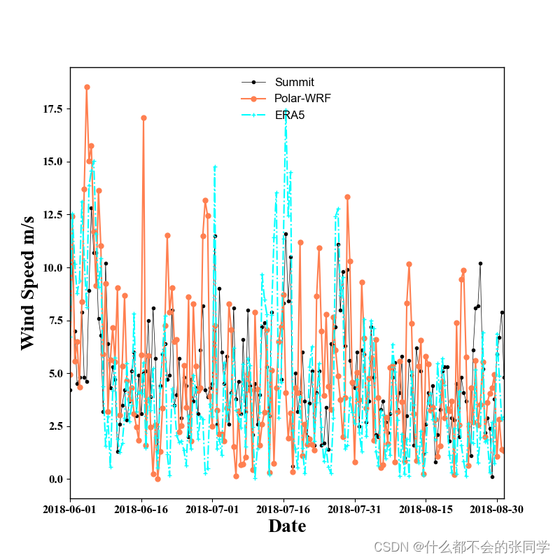
时间序列点线图——站点与模拟对比

将WRF的结果、再分析资料与站点观测数据对比，以点线图形式给出，由于比较简单，这里没有封装，主要是一些细节的设置需要记录：

#根据时间戳绘图
fig2 = plt.figure(figsize=(8,8))#设置画布大小
plt.plot(times,wdir_bar,marker='.',linestyle='-', linewidth = 0.5, label=st[nn], color='black')
plt.plot(times,uvmet10,marker='o', markersize=5, linestyle='-', label='Polar-WRF', color='coral')
plt.plot(times,met_uv10,marker='+', markersize=5, linestyle='-.', label='ERA5', color='aqua')
font1 = {'family' : 'Times New Roman',
    'weight' : 'bold',
    'size' : 20,
    }
plt.ylabel("Wind Speed m/s",font1)
plt.xlabel('Date',font1)
plt.xlim(np.min(times), np.max(times))
dates=pd.date_range(np.min(times), np.max(times),freq='15D')
plt.xticks(dates,fontproperties='Times New Roman', size=12,weight='bold')
plt.yticks(fontproperties='Times New Roman', size=12,weight='bold')
plt.legend(loc='upper center',frameon=False)
plt.show()

绘图：

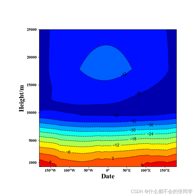
垂直剖面图

垂直剖面图（cross-section），也可以称作切片图，主要是将多维数据沿其中一维切片，将其绘出。
在气象中，可以绘制纬向、经向、时间剖面，即以经度、纬度或者时间为x轴，气象层或者高度层为y层，通过垂直剖面图，可以了解一个剖面的平行分布，如：绘制纬向平均时，我们可以知道各经度某一气象要素的垂直分布。
绘图函数：

def  cross_section(x,y,z,invert,levels,axis):#
    #选择剖面：纬向or经向,axis=1：经向.axis=2，纬向
    if len(np.shape(z))==4:
        z3d=np.mean(z,axis=axis+1) #z3d为时间×高度×经度or纬度的三维数组
        z2d=np.mean(z3d,axis=2)
        z2d=np.transpose(z2d)
    #3d切片
    if len(np.shape(z))==3:
        z2d=np.mean(z,axis=axis)#z2d为高度
    fig=plt.figure(figsize=(8,8))
    ax=fig.add_axes([0.2, 0.15, 0.7, 0.7])
    if invert==1: #是否翻转y轴
        ax.invert_yaxis()
    ca=ax.contourf(x,y,z2d,cmap=cmaps.matlab_jet,levels=10)
    line=ax.contour(x,y,z2d,levels=10,colors='black',linestyles='dashed',linewidths=1.0)
    plt.clabel(line,inline=True, fontsize=12,colors='black')
    plt.xticks(fontproperties='Times New Roman', size=12,weight='bold')
    plt.yticks(fontproperties='Times New Roman', size=12,weight='bold')
    plt.xlim(np.min(x), np.max(x))
    plt.ylim(np.min(y), 25000)
    return fig,ax,ca,line

调用绘图脚本，绘制北极地区夏季纬向温度垂直剖面：

level=np.mean(az,axis=1)
level=np.mean(level,axis=1）
lat=np.linspace(np.min(lat2d),np.max(lat2d),219)
lon=np.linspace(np.min(lon2d),np.max(lon2d),219)
fig,ax,ca,line=cross_section(lon,level,to_np(tk)-273.3,0,10,2)
font1 = {'family' : 'Times New Roman',
     'weight' : 'bold',
     'size' : 20,
     }
ax.set_xlabel('Date',font1)
ax.set_ylabel('Height/m',font1)
ax.set_yticks([25000,20000,15000,10000,5000,1000],fontproperties='Times New Roman', size=12,weight='bold')
ax.xaxis.set_major_formatter(cticker.LongitudeFormatter())
#dates=pd.date_range(np.min(times), np.max(times),freq='15D')
#ax.set_xticks(dates,fontproperties='Times New Roman', size=12,weight='bold')
plt.show()

气象场/风场

请参考本人另一篇博客；
python cartipy绘制北极气象场
与python cartipy绘制北极nc可视化

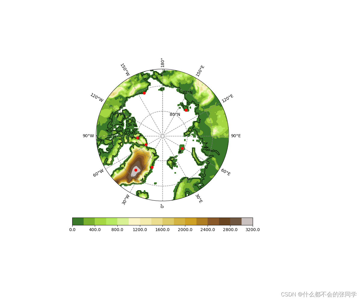
地形与站点绘制

将拥有的气象站绘制到模拟区域中，主要使用plot直接绘制：

stlat=[71.3,72.6,76.8,80.6,76.0,82.5,79.9]
stlon=[-156.8,-38.4,-18.7,58.1,137.9,-62.3,-85.9]
#绘制模拟区域地形
proj =ccrs.NorthPolarStereo(central_longitude=0)#设置地图投影
#在圆柱投影中proj = ccrs.PlateCarree(central_longitude=xx)
leftlon, rightlon, lowerlat, upperlat = (-180,180,60,90)#经纬度范围

img_extent = [leftlon, rightlon, lowerlat, upperlat]
fig1 = plt.figure(figsize=(12,10))#设置画布大小
f1_ax1 = fig1.add_axes([0.2, 0.3, 0.5, 0.5],projection = ccrs.NorthPolarStereo(central_longitude=0))#绘制地图位置
#注意此处添加了projection = ccrs.NorthPolarStereo()，指明该axes为北半球极地投影
#f1_ax1.gridlines(crs=ccrs.PlateCarree(), draw_labels=True,
 #                 linewidth=1, color='grey',linestyle='--')
f1_ax1.set_extent(img_extent, ccrs.PlateCarree())
f1_ax1.add_feature(cfeature.COASTLINE.with_scale('110m'))
lat2d=to_np(lats)
lon2d=to_np(lons)
ter=to_np(ter)
ter=np.ma.masked_values(ter, 0)
g1=f1_ax1.gridlines(crs=ccrs.PlateCarree(), draw_labels=True, linewidth=1, color='gray',linestyle='--')
X, Y, masked_MDT = z_masked_overlap(
    f1_ax1, lon2d, lat2d, ter,
    source_projection=ccrs.Geodetic())
g1.xlocator = mticker.FixedLocator(np.linspace(-180,180,13))
g1.ylocator = mticker.FixedLocator(np.linspace(60, 90,4))

theta = np.linspace(0, 2*np.pi, 100)
center, radius = [0.5, 0.5], 0.44
verts = np.vstack([np.sin(theta), np.cos(theta)]).T
circle = mpath.Path(verts * radius + center)
f1_ax1.set_boundary(circle, transform=f1_ax1.transAxes)
levels=np.arange(0,3300,200)
c7=f1_ax1.contourf(X, Y, masked_MDT,cmap=cmaps.OceanLakeLandSnow,levels=levels)
#quiver = f1_ax1.quiver(X, Y, u_500, v_500, pivot='tail',width=0.002, scale=200, color='black', headwidth=4,regrid_shape=30,alpha=1)
#f1_ax1.quiverkey(quiver, 0.91, 1.03, 5, "5m/s",labelpos='E', coordinates='axes', fontproperties={'size': 10,'family':'Times New Roman'})
position=fig1.add_axes([0.2, 0.25, 0.5, 0.025])#图标位置
font = {'family' : 'serif',
        'color'  : 'darkred',
        'weight' : 'normal',
        'size'   : 16,
        }
cb=fig1.colorbar(c7,cax=position,orientation='horizontal',format='%.1f',extend='both')#设置图标
#绘制站点
f1_ax1.plot(stlon,stlat, 'o', markersize=6, color='red',label='Station', transform=ccrs.Geodetic())
#cb.set_label('m',fontdict=font) #添加图标标签
plt.show()