论文笔记 PCL: Proposal Cluster Learning for Weakly Supervised Object Detection - TPAMI 2018

2018 PCL Proposal Cluster Learning for Weakly Supervised Object Detection

唐芃, 王兴刚 TPAMI, 2018 PDF | code

Abstract

作者在OICR的基础上，提出了使用区域聚类proposal clusters的方法学习细化分类器(refined instance classifiers, refined classifiers)。从个人看完会议论文OICR再看该期刊论文的感受，该(期刊)论文各种细节解释的比会议论文详细好多，但是还是存在一个没有搞懂的地方，由于个人对该论文还是比较感兴趣的，所以在后面会阅读代码，在阅读完之后再来对该博文欠缺之处做出修改 相关问题已在阅读源码后在后面对应疑惑处给出正确理解。

In this paper, we propose a novel deep network for WSOD. Unlike previous networks that transfer the object detection problem to an image classification problem using Multiple Instance Learning (MIL), our strategy generates proposal clusters to learn refined instance classifiers by an iterative process. The proposals in the same cluster are spatially adjacent and associated with the same object. This prevents the network from concentrating too much on parts of objects instead of whole objects. We first show that instances can be assigned object or background labels directly based on proposal clusters for instance classifier refinement, and then show that treating each cluster as a small new bag yields fewer ambiguities than the directly assigning label method. The iterative instance classifier refinement is implemented online using multiple streams in convolutional neural networks, where the first is an MIL network and the others are for instance classifier refinement supervised by the preceding one.

1. Introduction

Fig. 3. (a) Conventional MIL networks transfer the instance classification (object detection) problem to a bag classification (image classification) problem. (b) We propose to generate proposal clusters and assign proposals the label of the corresponding object class for each cluster. © We propose to treat each proposal cluster as a small new bag.“0”,“1”, and“2” indicate the “background”,“motorbike”, and“car”, respectively.

3. Method

Fig. 4. The architecture of our method. All arrows are utilized during the forward process of training, only the solid ones have back-propagation computations, and only the blue ones are used during testing. During the forward process of training, an image and its proposal boxes are fed into the CNN which involves a series of convolutional layers, an SPP layer, and two fully connected layers to produce proposal features. These proposal features are branched into many streams: the first one for the basic MIL network and the other ones for iterative instance classifier refinement. Each stream outputs a set of proposal scores and generates proposal clusters consequently. Based on these proposal clusters, supervisions are generated to compute losses for the next stream. During the back-propagation process of training, proposal features and classifiers are trained according to the network losses. All streams share the same proposal features.

The overall architecture of our method is shown in Fig. 4. Given an image, about 2, 000 object proposals from Selective Search or EdgeBox are generated. During the forward process of training, the image and these proposals are fed into some convolutional (conv) layers with an SPP layer to produce a fixed-size conv feature map per-proposal. After that, proposal feature maps are fed into two fully connected (fc) layers to produce proposal features. These features are branched into different streams: the first one is an MIL network to train basic instance classifiers and the others refine the classifiers iteratively. For each stream, proposal classification scores are obtained and proposal clusters are generated consequently. Then based on these proposal clusters, supervisions are generated to compute losses for the next stream. During the back-propagation process of training, the network losses are optimized to train proposal features and classifiers. As shown in the figure, supervisions of the $1$-st refined classifier depend on the output from the basic classifier, and supervisions of $k$-th refined classifier depend on outputs from { k − 1 } \{k− 1\} {k−1}-th refined classifier. In this section, we will introduce our method of learning refined instance classifiers based on proposal clusters in detail.

3.1 Notations

Before presenting our method, we first introduce some of the mostly used notations as follows. We have $R$ proposals with boxes B = { b r } r = 1 R \mathcal{B}=\left\{b_{r}\right\}_{r=1}^{R} B={br​}r=1R​ for an given image and proposal features $\mathbf{F}$, where $b_r$ is the $r$-th proposal box. The number of refined instance classifiers is $K$ (i.e., we refine instance classifier $K$ times), and thus there are $K+1$ streams. The number of object classes is $C.{\mathbf{W}}^0$ and W k , k ∈ { 1 , … , K } \mathbf{W}^{k}, k \in\{1, \ldots, K\} Wk,k∈{1,…,K} are the parameters of the basic instance classifier and the $k$-th refined instance classifier, respectively. ${\phi }^0\left(\mathbf{F},{\mathbf{W}}^0\right)\in$ ${\mathbb{R}}^{C\times R}$ and φ k ( F , W k ) ∈ R ( C + 1 ) × R , k ∈ { 1 , … , K } \varphi^{k}\left(\mathbf{F}, \mathbf{W}^{k}\right) \in \mathbb{R}^{(C+1) \times R}, k \in\{1, \ldots, K\} φk(F,Wk)∈R(C+1)×R,k∈{1,…,K} are the predicted score matrices of the basic instance classifier and the $k$-th refined instance classifier, respectively, where $C+1$ indicates the $C$ object classes and $1$ background class. We use ${\phi }^k$ later for simplification, dropping the dependence on $\mathbf{F},{\mathbf{W}}^k\cdot {\phi }_{cr}^k$ is the predicted score of the $r$-th proposal for class $c$ from the $k$-th instance classifier. $\mathbf{y}={\left[y_1,\dots ,y_C\right]}^T$ is the image label vector, where $y_c=1$ or 0 indicates the image with or without object class $c$. ${\mathcal{H}}^k\left({\mathbf{\phi }}^{k-1},\mathbf{y}\right)$ is the supervision of the $k$-th instance classifier, where ${\mathcal{H}}^k\left({\phi }^{k-1},\mathbf{y}\right),k=0$ is the image label vector $\mathbf{y}$. ${\mathrm{L}}^k\left(\mathbf{F},{\mathbf{W}}^k,{\mathcal{H}}^k\left({\mathbf{\phi }}^{k-1},\mathbf{y}\right)\right)$ is the loss function to train the $k$-th instance classifier.

We compute $N^k$ proposal cluster centers ${\mathcal{S}}^k={\left\{S_n^k\right\}}_{n=1}^{N^k}$ for the $k$-th refinement. The $n$-th cluster center $S_n^k=$ $\left(b_n^k,y_n^k,s_n^k\right)$ consists of a proposal box $b_n^k\in \mathcal{B}$, an object label y n k ( y n k = c , c ∈ { 1 , … , C } y_{n}^{k}\left(y_{n}^{k}=c, c \in\{1, \ldots, C\}\right. ynk​(ynk​=c,c∈{1,…,C} indicates the $c$-th object class), and a confidence score $s_i^k$ indicating the confidence that $b_n^k$ covers at least part of an object of class $y_n^k$. We have $N^k+1$ proposal clusters ${\mathcal{C}}^k={\left\{{\mathcal{C}}_n^k\right\}}_{n=1}^{N^k+1}$ according to ${\mathcal{S}}^k({\mathcal{C}}_{N^k+1}^k$ for background and others for objects). For object clusters, the $n$-th cluster ${\mathcal{C}}_n^k=\left({\mathcal{B}}_n^k,y_n^k,s_n^k\right),n\ne N^k+1$ consists of $M_n^k$ proposal boxes ${\mathcal{B}}_n^k={\left\{b_{nm}^k\right\}}_{m=1}^{M_n^k}\subseteq \mathcal{B}$, an object label $y_n^k$ that is the same as the cluster center label, and a confidence score $s_n^k$ that is the same as the cluster center score, where $s_n^k$ indicates the confidence that ${\mathcal{C}}_n^k$ corresponds to an object of class $y_n^k$. Unlike object clusters, the background cluster ${\mathcal{C}}_n^k=\left({\mathcal{P}}_n^k,y_n^k\right),n=N^k+1$ consists of $M_n^k$ proposals ${\mathcal{P}}_n^k={\left\{P_{nm}^k\right\}}_{m=1}^{M_n^k}$ and a label $y_n^k=C+1$ indicating the background. The $m$-th proposal $P_{nm}^k=\left(b_{nm}^k,s_{nm}^k\right)$ consists of a proposal box $b_{nm}^k\in \mathcal{B}$ and a confidence score $s_{nm}^k$ indicating the confidence that $b_{nm}^k$ is the background.

3.2 Basic MIL network

第一个细化分类器(即Fig.4.的Stream2)需要基本实例分类器来生成proposal scores和clusters作为监督。作者提出的PCL独立于特定的MIL方法，因此可以应用在所有端到端训练的MIL网络。在这里，由于作者在CVPR 2017发表的OICR使用WSDDN作为基础MIL网络，在PCL中，作者自然而然地使用了WSDDN作为基础MIL网络。为了论文的完备，作者在这里简要的介绍了WSDDN，在之前的博文中我也简要地介绍了WSDDN，在这里我直接复制原文作为参考，如果看不懂地可以参见我之前的博文。

Given an input image and its proposal boxes $\mathcal{B}=$ { b r } r = 1 R \left\{b_{r}\right\}_{r=1}^{R} {br​}r=1R​, a set of proposal features $\mathbf{F}$ are first generated by the network. Then as shown in the “Basic MIL network” block of Fig. 4, there are two branches which process the proposal features to produce two matrices ${\mathbf{X}}^{\text{cls }}\left(\mathbf{F},{\mathbf{W}}^{\text{cls }}\right),{\mathbf{X}}^{\text{det }}\left(\mathbf{F},{\mathbf{W}}^{\text{det }}\right)\in {\mathbb{R}}^{C\times R}$ (we use ${\mathbf{X}}^{\text{cls }},{\mathbf{X}}^{\text{det }}$ later for simplification, dropping the dependence on $\mathbf{F},{\mathbf{W}}^{\text{cls }},{\mathbf{W}}^{\text{det }}$ ) of an input image by two fc layers, where ${\mathbf{W}}^{\text{cls }}$ and ${\mathbf{W}}^{\text{det }}$ denote the parameters of the fc layer for ${\mathbf{X}}^{\mathrm{c}\mathrm{l}\mathrm{s}}$ and the parameters of the fc layer for ${\mathbf{X}}^{\mathrm{d}\mathrm{e}\mathrm{t}}$, respectively. Then the two matrices are passed through two softmax layer along different directions: ${\left[\mathbf{\sigma }\left({\mathbf{X}}^{\mathrm{c}\mathrm{l}\mathrm{s}}\right)\right]}_{cr}=e^{x_{cr}^{\mathrm{c}\mathrm{l}\mathrm{s}}}/{\sum }_{c^{\prime }=1}^C{e}^{x_{c^{\prime }r}^{\mathrm{c}\mathrm{l}\mathrm{s}}}$ and ${\left[\mathbf{\sigma }\left({\mathbf{X}}^{\mathrm{d}\mathrm{e}\mathrm{t}}\right)\right]}_{cr}=e^{x_{cr}^{\mathrm{d}\mathrm{e}\mathrm{t}}}/{\sum }_{r^{\prime }=1}^R{e}^{x_{c{r}^{\prime }}^{\mathrm{d}\mathrm{e}\mathrm{t}}}$. Let us denote $\left({\mathbf{W}}^{\mathrm{c}\mathrm{l}\mathrm{s}},{\mathbf{W}}^{\text{det }}\right)$ by ${\mathbf{W}}^0$. The proposal scores are generated by element-wise product ${\phi }^0\left(\mathbf{F},{\mathbf{W}}^0\right)=$ $\mathbf{\sigma }\left({\mathbf{X}}^{\mathrm{c}\mathrm{l}\mathrm{s}}\right)\odot \mathbf{\sigma }\left({\mathbf{X}}^{\mathrm{d}\mathrm{e}\mathrm{t}}\right)$. Finally, the image score of the $c$-th class ${\left[\varphi \left(\mathbf{F},{\mathbf{W}}^0\right)\right]}_c$ is obtained by the sum over all proposals: ${\left[\varphi \left(\mathbf{F},{\mathbf{W}}^0\right)\right]}_c={\sum }_{r=1}^R{\left[{\mathbf{\phi }}^0\left(\mathbf{F},{\mathbf{W}}^0\right)\right]}_{cr}.$

A simple interpretation of the two branches framework is as follows. ${\left[\mathbf{\sigma }\left({\mathbf{X}}^{\mathrm{c}\mathrm{l}\mathrm{s}}\right)\right]}_{cr}$ is the probability of the r-th proposal belonging to class c. ${\left[\mathbf{\sigma }\left({\mathbf{X}}^{\mathrm{d}\mathrm{e}\mathrm{t}}\right)\right]}_{cr}$ is the normalized weight that indicates the contribution of the r-th proposal to image being classified to class i. So ${\left[\varphi \left(\mathbf{F},{\mathbf{W}}^0\right)\right]}_c$ is obtained by weighted sum pooling and falls in the range of $(0,1)$. Given the image label vector $y=[y_1,...,y_C{]}^T$ . We train the basic instance classifier by optimizing the multi-class cross entropy loss $\text{Eq}.(1)$ w.r.t. $\mathbf{F},{\mathbf{W}}^0$.
$${\mathrm{L}}^0\left(\mathbf{F},{\mathbf{W}}^0,\mathbf{y}\right)=-\sum _{c=1}^C\{\left(1-y_c\right)\log \left(1-{\left[\mathbf{\varphi }\left(\mathbf{F},{\mathbf{W}}^0\right)\right]}_c\right)+y_c\log {\left[\mathbf{\varphi }\left(\mathbf{F},{\mathbf{W}}^0\right)\right]}_c\}$$

3.3 The overall training strategy

在Fig. 4.中，除第一个基础MIL网络(basic instance classifier)的所有Stream都对应着细化分类器。作者将基本 MIL 网络和细化分类器集成到端到端网络中，以在线学习细化分类器。同基础的MIL网络输出的分数矩阵${\phi }^0\left(\mathbf{F},{\mathbf{W}}^0\right)\in {\mathbb{R}}^{C\times R}$不同，$K$个细化分类器输出的分数矩阵 φ k ( F , W 0 ) ∈ R ( C + 1 ) × R , k ∈ { 1 , 2 , … , K } \varphi^{k}\left(\mathbf{F}, \mathbf{W}^{0}\right)\in\mathbb{R}^{(C+1)\times R}, k \in\{1,2, \ldots, K\} φk(F,W0)∈R(C+1)×R,k∈{1,2,…,K}，这是因为细化分类器的输出类别包含背景类别，具有 { C + 1 } \{C+1\} {C+1}个类别（这一点与OICR一致，同上所述，PCL是OICR的一个延伸版本，但在PCL中，作者也详细地介绍了PCL实现细节，所以个人觉得OICR可看可不看）。从${\mathbf{\phi }}^k\left(\mathbf{F},{\mathbf{W}}^k\right)$可以注意到，与${\phi }^0\left(\mathbf{F},{\mathbf{W}}^0\right)$相同，细化分类器使用了与基础MIL网络一样的特征$\mathbf{F}$。

第 k , k ∈ { 1 , … , K } k,k\in\{1,\dots,K\} k,k∈{1,…,K}的细化分类器监督${\mathcal{H}}^k\left({\mathbf{\phi }}^{k-1},\mathbf{y}\right)$产生于第$k-1$个分类器，由第$k-1$个分类器的得分矩阵${\mathbf{\phi }}^{k-1}$以及图像标签$\mathbf{y}={\left[y_1,\dots ,y_C\right]}^T$生成。监督${\mathcal{H}}^k\left({\mathbf{\phi }}^{k-1},\mathbf{y}\right)$不产生损失，即监督${\mathcal{H}}^k\left({\mathbf{\phi }}^{k-1},\mathbf{y}\right)$只在正向传播中计算，不参与梯度反向传播。结合基础MIL网络，PCL的总损失 $\text{Eq}.(2)$ 可写作：
$$\sum _{k=0}^K{\mathrm{L}}^k\left(\mathbf{F},{\mathbf{W}}^k,{\mathcal{H}}^k\left({\mathbf{\phi }}^{k-1},\mathbf{y}\right)\right)$$
对于$K$个细化分类器的损失${\mathrm{L}}^k\left(\mathbf{F},{\mathbf{W}}^k,{\mathcal{H}}^k\left({\mathbf{\phi }}^{k-1},\mathbf{y}\right)\right),k>0$ 将在 Section 3.4 $\text{Eq}.(6)/(7)/(8)$ 给出。

During the forward process of each Stochastic Gradient Descent (SGD) training iteration, we obtain a set of proposal scores of an input image. Accordingly, we generate the supervisions ${\mathcal{H}}^k\left({\mathbf{\phi }}^{k-1},\mathbf{y}\right)$ for the iteration to compute the loss $\text{Eq}.(2)$. During the back-propagation process of each SGD training iteration, we optimize the loss $\text{Eq}.(2)$ w.r.t. proposal features $\mathbf{F}$ and classifiers ${\mathbf{W}}^k$. We summarize this procedure in Algorithm 1. Note that we do not use an alternating training strategy, i.e.,fixing supervisions and training a complete model,fixing the model and updating supervisions. The reasons are that: 1) it is very time-consuming because it requires training models multiple times; 2) training different models in different refinement steps separately may harm the performance because it hinders the process to benefit from the shared proposal features (i.e., $\mathbf{F}$).

3.4 Proposal cluster learning

Here we will introduce our methods to learn refined instance classifiers based on proposal clusters (i.e., proposal cluster learning).

Recall from Section 3.1 that we have a set of proposals with boxes B = { b r } r = 1 R \mathcal{B}=\left\{b_{r}\right\}_{r=1}^{R} B={br​}r=1R​. For the $k$-th refinement, our goal is to generate supervisions ${\mathcal{H}}^k\left({\phi }^{k-1},\mathbf{y}\right)$ for the loss functions ${\mathrm{L}}^k\left(\mathbf{F},{\mathbf{W}}^k,{\mathcal{H}}^k\left({\mathbf{\phi }}^{k-1},\mathbf{y}\right)\right)$ using the proposal scores ${\phi }^{k-1}$ and image label $\mathbf{y}$ in each training iteration. We use ${\mathcal{H}}^k,{\mathrm{L}}^k$ later for simplification, dropping the dependence on ${\mathbf{\phi }}^{k-1},\mathbf{y},\mathbf{F},{\mathbf{W}}^k$.

We do this in three steps. 1) We find proposal cluster centers which are proposals corresponding to different objects. 2) We group the remaining proposals into different clusters, where each cluster is associated with a cluster center or corresponds to the background. 3) We generate the supervisions ${\mathcal{H}}^k$ for the loss functions ${\mathrm{L}}^k$, enabling us to train the refined instance classifiers.

For the first step, we compute proposal cluster centers ${\mathcal{S}}^k={\left\{S_n^k\right\}}_{n=1}^{N^k}$ based on ${\phi }^{k-1}$ and $\mathbf{y}$. The $n$-th cluster center $S_n^k=\left(b_n^k,y_n^k,s_n^k\right)$ is defined in Section 3.1. We propose two algorithms to find ${\mathcal{S}}^k$ in Section 3.4.1 (1) and (2) (also Algorithm 2 and Algorithm 3), where the first one was proposed in the conference version paper and the second one is proposed in this paper.

For the second step, according to the proposal cluster centers ${\mathcal{S}}^k$, proposal clusters ${\mathcal{C}}^k={\left\{{\mathcal{C}}_n^k\right\}}_{n=1}^{N^k+1}$ are generated (${\mathcal{C}}_{N^k+1}^k$ for background and others for objects). The $n$-th object cluster ${\mathcal{C}}_n^k=\left({\mathcal{B}}_n^k,y_n^k,s_n^k\right),n\ne N^k+1$ and the background cluster ${\mathcal{C}}_n^k=\left({\mathcal{P}}_n^k,y_n^k\right),n=N^k+1$ are defined in Section 3.1. We use the different notation for the background cluster because background proposals are scattered in each image, and thus it is hard to determine a cluster center and accordingly a cluster score. The method to generate ${\mathcal{C}}^k$ was proposed in the conference version paper and is described in Section 3.4.2 (also Algorithm 4).

For the third step, supervisions ${\mathcal{H}}^k$ to train the $k$-th refined instance classifier are generated based on the proposal clusters. We use two strategies where ${\mathcal{H}}^k$ are either proposal-level labels indicating whether a proposal belongs to an object class, or cluster-level labels that treats each proposal cluster as a bag. Subsequently these are used to compute the loss functions ${\mathrm{L}}^k$. We propose two approaches to do this as described in Section 3.4.3 (1) and (2), where the first one was proposed in the conference version paper and the second one is proposed in this paper.

3.4.1 Finding proposal cluster centers

在这个部分，作者介绍了两种proposal cluster centers的方法，分别对应Algorithm 2和Algorithm 3。

(1) Finding proposal cluster centers using the highest scoring proposal.

一个寻找proposal cluster centers的方案是，选择分数矩阵${\mathbf{\phi }}^{k-1}$中得分最高的建议区域作为proposal cluster centers。参考Algorithm 2，假定一张图片含有的目标类别$c$(i.e. $y_c=1$)，对于第$k$个细化分类器，按照 $\text{Eq}.(3)$ 选取第 $r_c^k$ 个建议区域作为 proposal cluster centers。
$$r_c^k=\underset{r}{\mathrm{argmax}}{\phi }_{cr}^{k-1}$$
所以有$S_n^k=\left(b_n^k,y_n^k,s_n^k\right)=\left(b_{r_c^k},c,{\phi }_{c{r}_c^k}^{k-1}\right)$，其中$b_{r_c^k}$表示第$r_c^k$个区域建议的边界框，${\phi }_{c{r}_c^k}^{k-1}$作为该蔟中心的信心分数（第$r_c^k$个提议至少涵盖$c$类对象的一部分），因为${\phi }_{c{r}_c^k}^{k-1}$是第$r_c^k$个区域建议被归类为$c$类的预测分数。

这样的处理存在一个潜在的问题，一个区域建议可能被多个类选作簇中心。对于这个问题，作者采用了一下方案，假定一个区域建议被多个类选作簇中心，则只保留预测分数最大的类，对其他类重新选择区域建议作为簇中心。There is a potential problem that one proposal may be chosen as the cluster centers for multiple object classes. To avoid this problem, if one proposal corresponds to the cluster centers for multiple object classes, this proposal would be chosen as the cluster center only by the class with the highest predicted score and we re-choose cluster centers for other classes.

(2) Finding proposal cluster centers using graphs of top ranking proposals.

使用预测得分最高的建议区域作为簇中心带来的另外一个问题是，在一张图片中，可能存在不止一个目标。这个也是OICR的一个问题所在，2019 CVPR有一篇文章(see this)就是以此为出发点做出了一些改进，应该还有其他相关的工作。针对这个问题，做题提出了基于图的方法选择簇中心。As stated in Section 1, although we can find good proposal cluster centers using the highest scoring proposal, this ignores that in natural images there are often more than one object for each category. Therefore, we propose a new method to find cluster centers using graphs of top ranking proposals.

对于$c$类，作者选择建议分数最高(with indexes ${\mathcal{R}}_c^k=\left\{r_{c1}^k,\dots ,r_{c{N}_c^k}^k\right\}$)的几个区域$V_c^k$建议作为无向图$G_c^k=\left(V_c^k,E_c^k\right)$的节点，当两个节点在空间上相邻(IoU大于某一阈值)时联通。More specifically, suppose an image has object class label $c$. We first select the top ranking proposals with indexes ${\mathcal{R}}_c^k=\left\{r_{c1}^k,\dots ,r_{c{N}_c^k}^k\right\}$ for the $k$-th refinement. Then we build an undirected unweighted graph $G_c^k=\left(V_c^k,E_c^k\right)$ of these proposals based on spatial similarity, where vertexes $V_c^k$ correspond to these top ranking proposals, and edges $E_c^k=\left\{e_{cr{r}^{\prime }}^k\right\}=\left\{e\left(v_{cr}^k,v_{c{r}^{\prime }}^k\right)\right\},r,r^{\prime }\in {\mathcal{R}}_c^k$ correspond to the connections between the vertexes. $e_{cr{r}^{\prime }}^k$ is determined according to the spatial similarity between two vertexes (i.e., proposals) as in $\text{Eq}.(4)$, where $I_{r{r}^{\prime }}$ is the IoU between the $r$-th and $r^{\prime }$-th proposals and $I_t$ is a threshold (e. g., 0.4).
$$e_{r{r}^{\prime }}=\{\begin{array}{ll}1& \text{ if }{I}_{r{r}^{\prime }}>I_t\\ 0& \text{ otherwise }\end{array}$$
我们贪婪地使用该图$G_c^k=\left(V_c^k,E_c^k\right)$为 $c$ 类生成一些聚类中心。也就是说，我们迭代地选择具有最多连接的顶点作为聚类中心，如Algorithm 3所示。在每次训练迭代中，每个图像的聚类中心的数量$N^k$都会发生变化，因为排名靠前的提议${\mathcal{R}}_c^k$会发生变化。有关$N^k$的一些实例，可参见Section 4.2.9。我们使用与Section 3.4.1 (1)相同的方法来避免选择一个提议作为多个对象类的聚类中心。（即对于一个区域建议可能被多个类选作簇中心的问题，只保留预测分数最大的类，对其他类重新选择区域建议作为簇中心。）Therefore, two vertexes are connected if they are spatially adjacent. After that, we greedily generate some cluster centers for class $c$ using this graph. That is, we iteratively select vertexes which have most connections to be the cluster centers, as in Algorithm 3. The number of cluster centers (i.e., $N^k$) changes for each image in each training iteration because the top ranking proposals ${\mathcal{R}}_c^k$ change. See Section 4.2.9 for some typical values of $N^k$. We use the same method as in Section 3.4.1 (1) to avoid one proposal been chosen as the cluster centers for multiple object classes.

采用这种策略的原因如下。首先，根据作者的观察，排名靠前的建议区域总是可以覆盖至少部分对象，因此从这些建议区域中生成簇中心可以鼓励选择的簇中心满足我们的要求。其次，因为这些建议区域很好地覆盖了对象，所以更好的建议区域（覆盖对象的更多部分）应该有更多的空间重叠建议区域（即有更多的连接）。第三，一些区域建议可以在空间上相去甚远，因此可以解决原OICR方法对于同一类别只能检测一个目标的问题。该方法还具有吸引人的特点，它可以为每个对象类生成自适应数量的建议区域，这是可取的，因为在正常的图像中每个类可以有任意数量的对象。作者将第$n$个提议聚类中心的信心分数$s_n^k$设置为(根据原问描述以及Algorithm 3，此处应为，对于类别$c$，将第$n$个提议聚类中心的信心分数$s_n^k$设置为)
$$s_n^k=\underset{r}{\max }{\phi }_{cr}^{k-1},r\text{ s.t. }{e}_{cr{r}_c^k}^k=1\text{ or }r=r_c^k$$
（参见Algorithm 3中的第 8 行），因为如果簇中心建议区域的相邻建议区域具有高置信度以覆盖对象的至少一部分（即具有高分类分数），则簇中心建议区域也应该具有如此高的置信度。

The reasons for this strategy are as follows. First, according to our observation, the top ranking proposals can always cover at least parts of objects, thus generating centers from these proposals encourages the selected centers to meet our requirements. Second, because these proposals cover objects well, better proposals (covering more parts of objects) should have more spatially overlapped proposals (i.e., have more connections). Third, these centers are spatially far apart, and thus different centers can correspond to different objects. This method also has the attractive characteristic that it can generate adaptive number of proposals for each object class, which is desirable because in natural images there are arbitrary number of objects per-class. We set the score of the $n$-th proposal cluster center $s_n^k$ by
$$s_n^k=\underset{r}{\max }{\phi }_{cr}^{k-1},r\text{ s.t. }{e}_{cr{r}_c^k}^k=1\text{ or }r=r_c^k$$
(see the 8-th line in Algorithm 3) because if the adjacent proposals of a center proposal have high confidence to cover at least part of an object (i.e., have high classification scores) the center proposal should also have such high confidence.

基于图的方法有一个重要问题：如何选择排名靠前的建议区域？一个简单的方法是选择分数超过阈值的提案。但在我们的案例中，建议区域分数在每次训练迭代中都会发生变化，因此很难确定阈值。相反，对于每个正对象类，我们使用 k-means 算法将图像的提案分数划分为一些聚类，并在聚类中选择得分中心最高的提案来形成排名靠前的提案。这种方法确保我们可以选择排名靠前的提案，尽管提案分数在训练期间会发生变化。其他选择是可能的，但这种方法在实验中效果很好。There is an important issue for the graph-based method: how to select the top ranking proposals? A simple method is to select proposals whose scores exceed a threshold. But in our case, proposal scores change in each training iteration, and thus it is hard to determine a threshold. Instead, for each positive object class, we use the k-means algorithm to divide proposal scores of an image into some clusters, and choose proposals in the cluster which has the highest score center to form the top ranking proposals. This method ensures that we can select the top ranking proposals although proposal scores change during training. Other choices are possible, but this method works well in experiments.

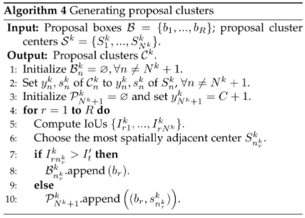
3.4.2 Generating proposal clusters

遍历每一个区域建议，计算该区域建议与其他区域建议的交并比，若交并比最大的区域是簇中心(with index $n_r^k$)且交并比大于某一阈值$I_t^{\prime }$，则将该区域建议添加进该簇中心对应的蔟；反之，归其为背景类对应的蔟，其信心分数为与其交并比最大的区域的信心分数（与其最相邻/交并比最大的区域有多大把握将自己归为某类，就有多大把握将靠近它的区域归为背景或者其他类）。

此处我有个疑问，在算法3中，对于$c$类拥有簇中心具有多个区域建议，每一个区域建议具有不一样的信心分数。但在生成蔟(算法4)的过程中，作者将该类$c$对应的蔟的信心分数设为同一个值？与算法3中一个簇中心可能具有多个信心分数有点出入？

根据作者GitHub的源代码，有多少个簇中心，就生成多少个蔟。我之前错误的理解为每个类只生成一个蔟，所以引发有多个簇中心导致信心分数不知如何选取的问题。原论文表达的是，每个蔟中心对应一个蔟，所以不涉及该问题。填坑完毕。

After the cluster centers are found, we generate the proposal clusters as in our conference version paper (OICR). Except for the cluster for background, good proposal clusters require that proposals in the same cluster are associated with the same object, and thus proposals in the same cluster should be spatially adjacent. Specially, given the $r$-th proposal, we compute a set of IoUs $\left\{I_{r1}^k,\dots ,I_{r{N}^k}^k\right\}$, where $I_{rn}^k$ is the IoU between the $r$-th proposal and the box $b_n^k$ of the $n$-th cluster center. Then we assign the $r$-th proposal to the $n_r^k$-th object cluster if $I_{r{n}_r^k}^k$ is larger than a threshold $I_t^{\prime }(e.g.,0.5)$ and to the background cluster otherwise, where $n_r^k$ is the index of the most spatially adjacent cluster center as $\text{Eq}.(5)$.
$$n_r^k=\underset{n}{\mathrm{argmax}}{I}_{rn}^k$$
The overall procedures to generate proposal clusters are summarized in Algorithm 4. We set the proposal scores for the background cluster to the scores of their most spatially adjacent centers as the 10-the line in Algorithm 4 , because if the cluster center $S_n^k$ has confidence $s_n^k$ that it covers an object, the proposal far away from $S_n^k$ should have confidence $s_n^k$ to be background.

3.4.3 Learning refined instance classifiers

在该部分，作者描述了如何计算细化分类器的损失。To get supervisions ${\mathcal{H}}^k$ and loss functions ${\mathrm{L}}^k$ to learn the $k$-th refined instance classifier, we design two approaches as follows.

(1) Assigning proposals object labels.

细化分类器的最直接方法是直接将对象标签分配给对象蔟中的所有区域建议，因为这些区域建议可能对应于整个对象，如我们的会议版本论文(OICR)中所示。由于蔟中心至少覆盖了部分对象，因此它们的相邻区域建议（即蔟中的提议）可以包含更大部分的对象。因此，我们可以将蔟标签 $y_n^k$ 分配给第 n 个集群中的所有区域建议。The most straightforward way to refine classifiers is to directly assign object labels to all proposals in object clusters because these proposals potentially correspond to whole objects, as in our conference version paper(OICR). As the cluster centers covers at least parts of objects, their adjacent proposals (i.e., proposals in the cluster) can contain larger parts of objects. Accordingly, we can assign the cluster label $y_n^k$ to all proposals in the $n$-th cluster.

More specifically, the supervisions ${\mathcal{H}}^k$ are proposal-level labels, i.e., ${\mathcal{H}}^k={\left\{{\mathbf{y}}_r^k\right\}}_{r=1}^R$. ${\mathbf{y}}_r^k={\left[y_{1r}^k,\dots ,y_{(C+1)r}^k\right]}^T\in {\mathbb{R}}^{(C+1)\times 1}$ is the label vector of the $r$-th proposal for the $k$ th refinement, where $y_{y_n^{k}r}^k=1$ and $y_{cr}^k=0,c\ne y_n^k$ if the $r$-th proposal belongs to the $n$-th clusters. Consequently, we use the standard softmax loss function to train the refined classifiers as in $\text{Eq}.(6)$, where ${\phi }_{cr}^k$ is the predicted score of the $r$-th proposal as defined in Section 3.1.
$${\mathrm{L}}^k\left(\mathbf{F},{\mathbf{W}}^k,{\mathcal{H}}^k\right)=-\frac{1}{R}\sum _{r=1}^R\sum _{c=1}^{C+1}{y}_{cr}^k\log {\phi }_{cr}^k$$
通过迭代实例分类器细化（即随着 k 的增加多次细化），检测器通过强制网络“看到”对象的较大部分来逐渐检测到对象的较大部分。Through iterative instance classifier refinement (i.e., multiple times of refinement as $k$ increase), the detector detects larger parts of objects gradually by forcing the network to “see” larger parts of objects.

与OICR相同，最靠前的几个细化分类器的预测效果是相对较差的，因此给每一个细化分类器权重相同权重是不合理的，故作者提出了一个加权版本，其出发点是，某个蔟如有很大的信心分数，其损失权重应该是大的，恰巧最靠前的几个细化分类器的预测的信心分数应该是小的，所以使用每个簇的信心分数最为其损失权重。Actually, the so learnt supervisions ${\mathcal{H}}^k$ are very noisy, especially in the beginning of training. This results in unstable solutions. To solve this problem, we change the loss in $\text{Eq}.(6)$ to a weighted version, as in $\text{Eq}.(7)$.
$${\mathrm{L}}^k\left(\mathbf{F},{\mathbf{W}}^k,{\mathcal{H}}^k\right)=-\frac{1}{R}\sum _{r=1}^R\sum _{c=1}^{C+1}{\lambda }_r^k{y}_{cr}^k\log {\phi }_{cr}^k$$
${\lambda }_r^k$ is the loss weight that is the same as the cluster confidence score $s_n^k$ for object clusters or proposal confidence score $s_{nm}^k$ for the background cluster if the $r$-th proposal belongs to the $n$-th cluster. From Algorithm 4, we can observe that ${\lambda }_r^k$ is the same as the cluster center confidence score $s_n^k$. The reasons for this strategy are as follows. In the beginning of training, although we cannot obtain good proposal clusters, each $s_n^k$ is small, hence each ${\lambda }_r^k$ is small and the loss is also small. As a consequence, the performance of the network will not decrease a lot. During the training, the top ranking proposals will cover objects well, and thus we can generate good proposal clusters. Then we can train satisfactory instance classifiers.

(2) Treating clusters as bags.

作者进一步对上述直接分配标签的方法计算损失函数进行修改，将每一个蔟视为bag。与直接分配标签的方法相比，该方法容忍了一些低分的建议区域，可以在一定程度上减少歧义。

As we stressed before, although directly assigning proposals object labels can boost the results, it may confuse the network because we simultaneously assign the same label to different parts of objects. Focusing on this, we further propose to treat each proposal cluster as a small new bag and use the cluster label as the bag label. Thus the supervisions ${\mathcal{H}}^k$ for the $k$-th refinement are bag-level (cluster-level) labels, i.e., ${\mathcal{H}}^k={\left\{y_n^k\right\}}_{n=1}^{N^k+1}$. $y_n^k$ is the label of the $n$-th bag, i.e., the label of the $n$-th proposal cluster, as defined in Section 3.1.

Specially, for object clusters, we choose average MIL pooling, because these proposals should cover at least parts of objects and thus should have relatively high prediction scores. For the background cluster, we assign the background label to all proposals in the cluster according to the MIL constraints (all instances in negative bags are negative). Then the loss function for refinement will be $\text{Eq}.(8)$.
$${\mathrm{L}}^k\left(\mathbf{F},{\mathbf{W}}^k,{\mathcal{H}}^k\right)=-\frac{1}{R}\left(\sum _{n=1}^{N^k}{s}_n^k{M}_n^k\log \frac{{\sum }_{r\text{ s.t. }{b}_r\in {\mathcal{B}}_n^k}{\phi }_{y_n^{k}r}^k}{M_n^k}+\sum _{r\in {\mathcal{C}}_{N^k+1}^k}{\lambda }_r^k\log {\phi }_{(C+1)r}^k\right)$$
$s_n^k$, $M_n^k$, and ${\phi }_{cr}^k$ are the cluster confidence score of the $n$-th object cluster, the number of proposals in the $n$-th cluster, and the predicted score of the $r$-th proposal, respectively, as defined in Section 3.1. $b_r\in {\mathcal{B}}_n^k$ and $r\in {\mathcal{C}}_{N^k+1}^k$ indicate that the $r$-th proposal belongs to the $n$-th object cluster and the background cluster respectively.

Compared with the directly assigning label approach, this method tolerates some proposals to have low scores, which can reduce the ambiguities to some extent.

3.5 Testing

During testing, the proposal scores of refined instance classifiers are used as the final detection scores, as the blue arrows in Fig. 4. Here the mean output of all refined classifiers is chosen. The Non-Maxima Suppression (NMS) is used to filter out redundant detections.

4 EXPERIMENTS

实验部分还是值得看一下的，这里我就不翻译了。

In this section, wefirst introduce our experimental setup including datasets, evaluation metrics, and implementation details. Then we conduct elaborate experiments to discuss the influence of different settings. Next, we compare our results with others to show the effectiveness of our method. After that, we show some qualitative results for further analyses. Finally, we give some runtime analyses of our method. Codes for reproducing our results are available at https://github.com/ppengtang/oicr/tree/pcl.

4.1 Experimental setup

4.1.1 Datasets and evaluation metrics

We evaluate our method on four challenging datasets: the PASCAL VOC 2007 and 2012 datasets [3], the ImageNet detection dataset [4], and the MS-COCO dataset [5]. Only image-level annotations are used to train our models.

The PASCAL VOC 2007 and 2012 datasets have 9, 962 and 22, 531 images respectively for 20 object classes. These two datasets are divided into train, val, and test sets. Here we choose the trainval set (5, 011 images for 2007 and 11, 540 images for 2012) to train our network. For testing, there are two metrics for evaluation: mAP and CorLoc. Following the standard PASCAL VOC protocol [3], Average Precision (AP) and the mean of AP (mAP) is the evaluation metric to test our model on the testing set. Correct Localization (CorLoc) is to test our model on the training set measuring the localization accuracy [34]. All these two metrics are based on the PASCAL criterion, i.e., IoU>0.5 between groundtruth boundingboxes and predicted boxes.

The ImageNet detection dataset has hundreds of thousands of images with 200 object classes. It is also divided into train, val, and test sets. Following [6], we split the val set into val1 and val2, and randomly choose at most 1K images in the train set for each object class (we call it train1K). We train our model on the mixture of train1K and val1 sets, and test it on the val2 set, which will lead to 160, 651 images for training and 9, 916 images for testing. We also use the mAP for evaluation on the ImageNet.

The MS-COCO dataset has 80 object classes and is divided into train, val, and test sets. Since the groundtruths on the test set are not released, we train our model on the MS-COCO 2014 train set (about 80K images) and test it on the val set (about 40K images). For evaluation, we use two metrics mAP@0.5 and mAP@[.5, .95] which are the standard PASCAL criterion (i.e., IoU>0.5) and the standard MS-COCO criterion (i.e., computing the average of mAP for IoU∈[0.5 : 0.05 : 0.95]) respectively.

4.1.2 Implementation details

Our method is built on two pre-trained ImageNet [4] networks VGG M [49] and VGG16 [50], each of which has some conv layers with max-pooling layers and three fc layers. We replace the last max-pooling layer by the SPP layer, and the last fc layer as well as the softmax loss layer by the layers described in Section 3. To increase the feature map size from the last conv layer, we replace the penultimate max-pooling layer and its subsequent conv layers by the dilated conv layers [51], [52]. The newly added layers are initialized using Gaussian distributions with 0-mean and standard deviations 0.01. Biases are initialized to 0.

During training, the mini-batch size for SGD is set to be 2, 32, and 4 for PASCAL VOC, ImageNet, and MSCOCO, respectively. The learning rate is set to 0.001 for thefirst 40K, 60K, 15K, and 85K iterations for the PASCAL VOC 2007, PASCAL VOC 2012, ImageNet, and MS-COCO datasets, respectively. Then we decrease the learning rate to 0.0001 in the following 10K, 20K, 5K, and 20K iterations for the PASCAL VOC 2007, PASCAL VOC 2012, ImageNet, and MS-COCO datasets, respectively. The momentum and weight decay are set to be 0.9 and 0.0005 respectively.

Selective Search [20], EdgeBox [47], and MCG [53] are adopted to generate about 2,000 proposals per-image for the PASCAL VOC, ImageNet, and MS-COCO datasets, respectively. For data augmentation, we use five image scales { 480 , 576 , 688 , 864 , 1200 } \{480,576,688,864,1200\} {480,576,688,864,1200} (resize the shortest side to one of these scales) with horizontal flips for both training and testing. If not specified, the instance classifiers are refined three times, i.e., $K=3$ in Section 3.3, so there are four output streams; the IoU threshold $I_t$ in Section 3.4.1 (2) (also Eq. (4)) is set to $0.4$; the number of $k$-means clusters in the last paragraph of Section 3.4.1 (2) is set to $3;I_t^{\prime }$ in Section 3.4.2 (also the 5-th line of Algorithm 4) is set to $0.5$.
Similar to other works [19],[43],[54], we train a supervised object detector through choosing the top-scoring proposals given by our method as pseudo groundtruths to further improve our results. Here we train a Fast R-CNN (FRCNN) [7] using the VGG16 model and the same five image scales (horizontal flips only in training). The same (with $30\%$ IoU threshold) is applied to compute AP.

Our experiments are implemented based on the Caffe [55] deep learning framework, using Python and C++. The $k$-means algorithm to produce top ranking proposals is implemented by scikit-learn [56]. All of our experiments are running on an NVIDIA GTX TitanX Pascal GPU and Intel® i7-6850K CPU (3.60GHz).

4.2 Discussions

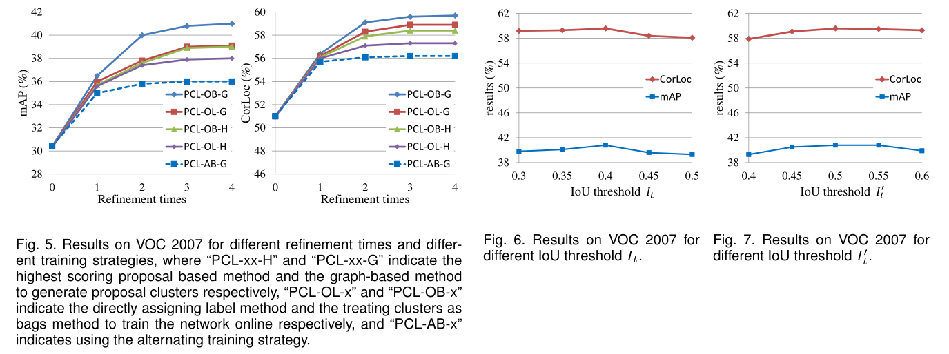
We first conduct some experiments to discuss the influence of different components of our method (including instance classifier refinement, different proposal generation methods, different refinement strategies, and weighted loss) and different parameter settings (including the IoU threshold It defined in Section 3.4.1 (2), the number of k-means clusters described in Section 3.4.1 (2), the IoU threshold I 0t defined in Section 3.4.2, and multi-scale training and testing.) We also discuss the number of proposal cluster centers. Without loss of generality, we only perform experiments on the VOC 2007 dataset and use the VGG M model.