OpenCV还能实现这种效果？视频防抖技术！

最新推荐文章于 2024-04-27 11:13:02 发布

爬遍天下无敌手

最新推荐文章于 2024-04-27 11:13:02 发布

阅读量1k

点赞数

分类专栏： Python 文章标签：算法 c++ python 计算机视觉 java

原文链接：https://blog.csdn.net/flyfor2013/article/details/108426811?utm_medium=distribute.pc_feed.none-task-blog-personrec_tag-9.nonecase&depth_1-utm_source=distribute.pc_feed.none-task-blog-personrec_tag-9.nonecase&request_id=5f5755f65361b606e50cbead

版权

Python 专栏收录该内容

1020 篇文章 166 订阅

订阅专栏

这篇文章分享了一个视频防抖的策略，这个方法同样可以应用到其他领域，比如常见的关键点检测，当使用视频测试时，效果就没有demo那么好，此时可以考虑本文的方法去优化。

分享这些demo并不一定所有人都会用到，但是在解决实际问题的时候，可以提供一个思路去解决问题。希望能给我一个三连，鼓励一下哈

在这篇文章中，我们将学习如何使用OpenCV库中的点特征匹配技术来实现一个简单的视频稳定器。我们将讨论算法并且会分享代码(python和C++版)，以使用这种方法在OpenCV中设计一个简单的稳定器。

视频中低频摄像机运动的例子

视频防抖是指用于减少摄像机运动对最终视频的影响的一系列方法。摄像机的运动可以是平移（比如沿着x、y、z方向上的运动）或旋转（偏航、俯仰、翻滚）。

视频防抖的应用

对视频防抖的需求在许多领域都有。

这在消费者和专业摄像中是极其重要的。因此，存在许多不同的机械、光学和算法解决方案。即使在静态图像拍摄中，防抖技术也可以帮助拍摄长时间曝光的手持照片。

在内窥镜和结肠镜等医疗诊断应用中，需要对视频进行稳定，以确定问题的确切位置和宽度。

同样，在军事应用中，无人机在侦察飞行中捕获的视频也需要进行稳定，以便定位、导航、目标跟踪等。同样的道理也适用于机器人。

视频防抖的不同策略

视频防抖的方法包括机械稳定方法、光学稳定方法和数字稳定方法。下面将简要讨论这些问题:

机械视频稳定：机械图像稳定系统使用由特殊传感器如陀螺仪和加速度计检测到的运动来移动图像传感器以补偿摄像机的运动。
光学视频稳定：在这种方法中，不是移动整个摄像机，而是通过镜头的移动部分来实现稳定。这种方法使用了一个可移动的镜头组合，当光通过相机的镜头系统时，可以可变地调整光的路径长度。
数字视频稳定：这种方法不需要特殊的传感器来估计摄像机的运动。主要有三个步骤:1）运动估计2）运动平滑，3）图像合成。第一步导出了两个连续坐标系之间的变换参数。第二步过滤不需要的运动，在最后一步重建稳定的视频。
在这篇文章中，我们将学习一个快速和鲁棒性好的数字视频稳定算法的实现。它是基于二维运动模型，其中我们应用欧几里得（即相似性）变换包含平移、旋转和缩放。

OpenCV Motion Models

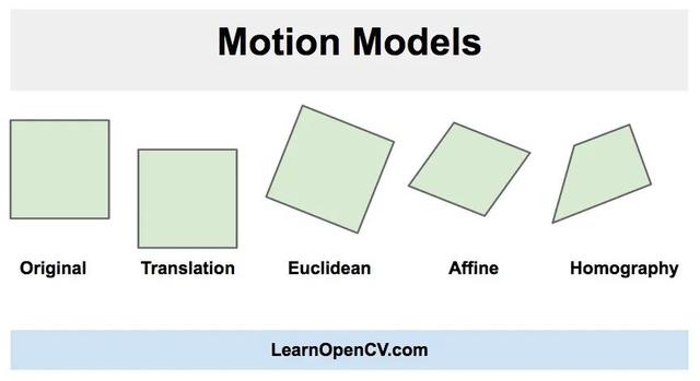
正如你在上面的图片中看到的，在欧几里得运动模型中，图像中的一个正方形可以转换为任何其他位置、大小或旋转不同的正方形。它比仿射变换和单应变换限制更严格，但对于运动稳定来说足够了，因为摄像机在视频连续帧之间的运动通常很小。

使用点特征匹配实现视频防抖

该方法涉及跟踪两个连续帧之间的多个特征点。跟踪特征允许我们估计帧之间的运动并对其进行补偿。

下面的流程图显示了基本步骤。

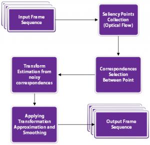
我们来看看这些步骤。

第一步：设置输入和输出视频

首先，让我们完成读取输入视频和写入输出视频的设置。代码中的注释解释每一行。

Python

# Import numpy and OpenCV
import numpy as np
import cv2
 
 
# Read input video
cap = cv2.VideoCapture('video.mp4')&nbsp;
 
 
# Get frame count
n_frames = int(cap.get(cv2.CAP_PROP_FRAME_COUNT)) 
 
 
# Get width and height of video stream
w = int(cap.get(cv2.CAP_PROP_FRAME_WIDTH)) 
h = int(cap.get(cv2.CAP_PROP_FRAME_HEIGHT))
 
 
# Define the codec for output video
fourcc = cv2.VideoWriter_fourcc(*'MJPG')
 
 
# Set up output video
out = cv2.VideoWriter('video_out.mp4', fourcc, fps, (w, h))

C++

 // Read input video
  VideoCapture cap("video.mp4");
 
 
  // Get frame count
  int n_frames = int(cap.get(CAP_PROP_FRAME_COUNT)); 
 
 
  // Get width and height of video stream
  int w = int(cap.get(CAP_PROP_FRAME_WIDTH)); 
  int h = int(cap.get(CAP_PROP_FRAME_HEIGHT));
 
 
  // Get frames per second (fps)
  double fps = cap.get(CV_CAP_PROP_FPS);
 
 
  // Set up output video
  VideoWriter out("video_out.avi", CV_FOURCC('M','J','P','G'), fps, Size(2 * w, h));

第二步：读取第一帧并将其转换为灰度图

对于视频稳定，我们需要捕捉视频的两帧，估计帧之间的运动，最后校正运动。

Python

# Read first frame
_, prev = cap.read() 
 
 
# Convert frame to grayscale
prev_gray = cv2.cvtColor(prev, cv2.COLOR_BGR2GRAY)

C++

 // Define variable for storing frames
  Mat curr, curr_gray;
  Mat prev, prev_gray;
 
 
  // Read first frame
  cap &gt;&gt; prev;
 
 
  // Convert frame to grayscale
  cvtColor(prev, prev_gray, COLOR_BGR2GRAY);

第三步：寻找帧之间的移动

这是算法中最关键的部分。我们将遍历所有的帧，并找到当前帧和前一帧之间的移动。没有必要知道每一个像素的运动。欧几里得运动模型要求我们知道两个坐标系中两个点的运动。但是在实际应用中，找到50-100个点的运动，然后用它们来稳健地估计运动模型是一个好方法。

3.1 可用于跟踪的优质特征
现在的问题是我们应该选择哪些点进行跟踪。请记住，跟踪算法使用一个小补丁围绕一个点来跟踪它。这样的跟踪算法受到孔径问题的困扰，如下面的视频所述

因此，光滑的区域不利于跟踪，而有很多角的纹理区域则比较好。幸运的是，OpenCV有一个快速的特征检测器，可以检测最适合跟踪的特性。它被称为goodFeaturesToTrack)

3.2 Lucas-Kanade光流
一旦我们在前一帧中找到好的特征，我们就可以使用Lucas-Kanade光流算法在下一帧中跟踪它们。

它是利用OpenCV中的calcOpticalFlowPyrLK函数实现的。在calcOpticalFlowPyrLK这个名字中，LK代表Lucas-Kanade，而Pyr代表金字塔。计算机视觉中的图像金字塔是用来处理不同尺度(分辨率)的图像的。

由于各种原因，calcOpticalFlowPyrLK可能无法计算出所有点的运动。例如，当前帧的特征点可能会被下一帧的另一个对象遮挡。幸运的是，您将在下面的代码中看到，calcOpticalFlowPyrLK中的状态标志可以用来过滤掉这些值。

3.3 估计运动
回顾一下，在3.1步骤中，我们在前一帧中找到了一些好的特征。在步骤3.2中，我们使用光流来跟踪特征。换句话说，我们已经找到了特征在当前帧中的位置，并且我们已经知道了特征在前一帧中的位置。所以我们可以使用这两组点来找到映射前一个坐标系到当前坐标系的刚性（欧几里德）变换。这是使用函数estimateRigidTransform完成的。

一旦我们估计了运动，我们可以把它分解成x和y的平移和旋转（角度）。我们将这些值存储在一个数组中，这样就可以平稳地更改它们。

下面的代码将完成步骤3.1到3.3。请务必阅读代码中的注释以进行后续操作。

Python

# Pre-define transformation-store array
transforms = np.zeros((n_frames-1, 3), np.float32) 
 
 
for i in range(n_frames-2):
  # Detect feature points in previous frame
  prev_pts = cv2.goodFeaturesToTrack(prev_gray,
                                     maxCorners=200,
                                     qualityLevel=0.01,
                                     minDistance=30,
                                     blockSize=3)
   
  # Read next frame
  success, curr = cap.read() 
  if not success: 
    break 
 
  # Convert to grayscale
  curr_gray = cv2.cvtColor(curr, cv2.COLOR_BGR2GRAY) 
 
  # Calculate optical flow (i.e. track feature points)
  curr_pts, status, err = cv2.calcOpticalFlowPyrLK(prev_gray, curr_gray, prev_pts, None) 
 
  # Sanity check
  assert prev_pts.shape == curr_pts.shape 
 
  # Filter only valid points
  idx = np.where(status==1)[0]
  prev_pts = prev_pts[idx]
  curr_pts = curr_pts[idx]
 
  #Find transformation matrix
  m = cv2.estimateRigidTransform(prev_pts, curr_pts, fullAffine=False) #will only work with OpenCV-3 or less
   
  # Extract traslation
  dx = m[0,2]
  dy = m[1,2]
 
  # Extract rotation angle
  da = np.arctan2(m[1,0], m[0,0])
   
  # Store transformation
  transforms[i] = [dx,dy,da]
   
  # Move to next frame
  prev_gray = curr_gray
 
 
  print("Frame: " + str(i) +  "/" + str(n_frames) + " -  Tracked points : " + str(len(prev_pts)))

C++

在c++实现中，我们首先定义一些类来帮助我们存储估计的运动向量。下面的TransformParam类存储了运动信息（dx -运动在x中，dy -运动在y中，da -角度变化），并提供了一个方法getTransform来将该运动转换为变换矩阵。

struct TransformParam
{
  TransformParam() {}
  TransformParam(double _dx, double _dy, double _da) 
  {
      dx = _dx;
      dy = _dy;
      da = _da;
  }
 
 
  double dx;
  double dy;
  double da; // angle
 
 
  void getTransform(Mat &amp;T)
{
    // Reconstruct transformation matrix accordingly to new values
    T.at&lt;double&gt;(0,0) = cos(da);
    T.at&lt;double&gt;(0,1) = -sin(da);
    T.at&lt;double&gt;(1,0) = sin(da);
    T.at&lt;double&gt;(1,1) = cos(da);
 
 
    T.at&lt;double&gt;(0,2) = dx;
    T.at&lt;double&gt;(1,2) = dy;
  }
};

在下面的代码中，我们循环视频帧并执行步骤3.1到3.3。

// Pre-define transformation-store array
  vector &lt;TransformParam&gt; transforms; 
 
 
  // 
  Mat last_T;
 
 
  for(int i = 1; i &lt; n_frames-1; i++)
  {
    // Vector from previous and current feature points
    vector &lt;Point2f&gt; prev_pts, curr_pts;
 
 
    // Detect features in previous frame
    goodFeaturesToTrack(prev_gray, prev_pts, 200, 0.01, 30);
 
 
    // Read next frame 
    bool success = cap.read(curr);
    if(!success) break; 
    
    // Convert to grayscale
    cvtColor(curr, curr_gray, COLOR_BGR2GRAY);
 
 
    // Calculate optical flow (i.e. track feature points)
    vector &lt;uchar&gt; status;
    vector &lt;float&gt; err;
    calcOpticalFlowPyrLK(prev_gray, curr_gray, prev_pts, curr_pts, status, err);
 
 
    // Filter only valid points
    auto prev_it = prev_pts.begin(); 
    auto curr_it = curr_pts.begin(); 
    for(size_t k = 0; k &lt; status.size(); k++) 
    {
        if(status[k]) 
        {
          prev_it++; 
          curr_it++; 
        }
        else 
        {
          prev_it = prev_pts.erase(prev_it);
          curr_it = curr_pts.erase(curr_it);
        }
    }
 
 
    
    // Find transformation matrix
    Mat T = estimateRigidTransform(prev_pts, curr_pts, false); 
 
 
    // In rare cases no transform is found. 
    // We'll just use the last known good transform.
    if(T.data == NULL) last_T.copyTo(T);
    T.copyTo(last_T);
 
 
    // Extract traslation
    double dx = T.at&lt;double&gt;(0,2);
    double dy = T.at&lt;double&gt;(1,2);
    
    // Extract rotation angle
    double da = atan2(T.at&lt;double&gt;(1,0), T.at&lt;double&gt;(0,0));
 
 
    // Store transformation 
    transforms.push_back(TransformParam(dx, dy, da));
 
 
    // Move to next frame
    curr_gray.copyTo(prev_gray);
 
 
    cout &lt;&lt; "Frame: " &lt;&lt; i &lt;&lt; "/" &lt;&lt; n_frames &lt;&lt; " -  Tracked points : " &lt;&lt; prev_pts.size() &lt;&lt; endl;
  }

第四步：计算帧之间的平滑运动

在前面的步骤中，我们估计帧之间的运动并将它们存储在一个数组中。我们现在需要通过叠加上一步估计的微分运动来找到运动轨迹。

步骤4.1:轨迹计算

在这一步，我们将增加运动之间的帧来计算轨迹。我们的最终目标是平滑这条轨迹。

Python 在Python中，可以很容易地使用numpy中的cumsum(累计和)来实现。

# Compute trajectory using cumulative sum of transformationstrajectory = np.cumsum(transforms, axis=0

C++

在c++中，我们定义了一个名为Trajectory的结构体来存储转换参数的累积和。

struct Trajectory
{
    Trajectory() {}
    Trajectory(double _x, double _y, double _a) {
        x = _x;
        y = _y;
        a = _a;
    }
 
 
    double x;
    double y;
    double a; // angle
};

C我们还定义了一个函数cumsum，它接受一个TransformParams 向量，并通过执行微分运动dx、dy和da(角度)的累积和返回轨迹。

vector&lt;Trajectory&gt; cumsum(vector&lt;TransformParam&gt; &amp;transforms)
{
  vector &lt;Trajectory&gt; trajectory; // trajectory at all frames
  // Accumulated frame to frame transform
  double a = 0;
  double x = 0;
  double y = 0;
 
 
  for(size_t i=0; i &lt; transforms.size(); i++) 
  {
      x += transforms[i].dx;
      y += transforms[i].dy;
      a += transforms[i].da;
 
 
      trajectory.push_back(Trajectory(x,y,a));
 
 
  }
 
 
  return trajectory; 
}

步骤4.2:计算平滑轨迹

在上一步中，我们计算了运动轨迹。所以我们有三条曲线来显示运动(x, y，和角度)如何随时间变化。

在这一步，我们将展示如何平滑这三条曲线。

平滑任何曲线最简单的方法是使用移动平均滤波器（moving average filter）。顾名思义，移动平均过滤器将函数在某一点上的值替换为由窗口定义的其相邻函数的平均值。让我们看一个例子。

假设我们在数组c中存储了一条曲线，那么曲线上的点是c[0]…c[n-1]。设f是我们通过宽度为5的移动平均滤波器过滤c得到的平滑曲线。

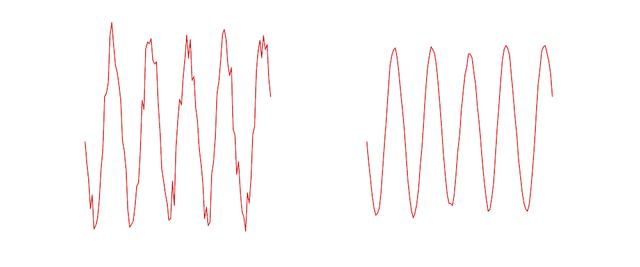
该曲线的k^{th}元素使用

如您所见，平滑曲线的值是噪声曲线在一个小窗口上的平均值。下图显示了左边的噪点曲线的例子，使用右边的尺度为5 滤波器进行平滑。

Python

在Python实现中，我们定义了一个移动平均滤波器，它接受任何曲线(即1-D的数字)作为输入，并返回曲线的平滑版本。

def movingAverage(curve, radius): 
  window_size = 2 * radius + 1
  # Define the filter 
  f = np.ones(window_size)/window_size 
  # Add padding to the boundaries 
  curve_pad = np.lib.pad(curve, (radius, radius), 'edge') 
  # Apply convolution 
  curve_smoothed = np.convolve(curve_pad, f, mode='same') 
  # Remove padding 
  curve_smoothed = curve_smoothed[radius:-radius]
  # return smoothed curve
  return curve_smoothed

我们还定义了一个函数，它接受轨迹并对这三个部分进行平滑处理。

def smooth(trajectory): 
  smoothed_trajectory = np.copy(trajectory) 
  # Filter the x, y and angle curves
  for i in range(3):
    smoothed_trajectory[:,i] = movingAverage(trajectory[:,i], radius=SMOOTHING_RADIUS)
 
 
  return smoothed_trajectory

这是最后去使用

# Compute trajectory using cumulative sum of transformations
trajectory = np.cumsum(transforms, axis=0)

C++

在c++版本中，我们定义了一个名为smooth的函数，用于计算平滑移动平均轨迹。

vector &lt;Trajectory&gt; smooth(vector &lt;Trajectory&gt;&amp; trajectory, int radius)
{
  vector &lt;Trajectory&gt; smoothed_trajectory; 
  for(size_t i=0; i &lt; trajectory.size(); i++) {
      double sum_x = 0;
      double sum_y = 0;
      double sum_a = 0;
      int count = 0;
 
 
      for(int j=-radius; j &lt;= radius; j++) { if(i+j &gt;= 0 &amp;&amp; i+j &lt; trajectory.size()) {
              sum_x += trajectory[i+j].x;
              sum_y += trajectory[i+j].y;
              sum_a += trajectory[i+j].a;
 
 
              count++;
          }
      }
 
 
      double avg_a = sum_a / count;
      double avg_x = sum_x / count;
      double avg_y = sum_y / count;
 
 
      smoothed_trajectory.push_back(Trajectory(avg_x, avg_y, avg_a));
  }
 
 
  return smoothed_trajectory; 
}

我们在主函数中使用它

// Smooth trajectory using moving average filter  vector &lt;Trajectory&gt; smoothed_trajectory = smooth(trajectory, SMOOTHING_RADIUS);

步骤4.3:计算平滑变换
到目前为止，我们已经得到了一个平滑的轨迹。在这一步，我们将使用平滑的轨迹来获得平滑的变换，可以应用到视频的帧来稳定它。

这是通过找到平滑轨迹和原始轨迹之间的差异，并将这些差异加回到原始的变换中来完成的。

Python

# Calculate difference in smoothed_trajectory and trajectory
difference = smoothed_trajectory - trajectory
 
# Calculate newer transformation array
transforms_smooth = transforms + difference

C++

vector <TransformParam> transforms_smooth;
for(size_t i=0; i < transforms.size(); i++)
{
// Calculate difference in smoothed_trajectory and trajectory
double diff_x = smoothed_trajectory[i].x - trajectory[i].x;
double diff_y = smoothed_trajectory[i].y - trajectory[i].y;
double diff_a = smoothed_trajectory[i].a - trajectory[i].a;
// Calculate newer transformation array
double dx = transforms[i].dx + diff_x;
double dy = transforms[i].dy + diff_y;
double da = transforms[i].da + diff_a;
transforms_smooth.push_back(TransformParam(dx, dy, da));
}

第五步:将平滑的摄像机运动应用到帧中

差不多做完了。现在我们所需要做的就是循环帧并应用我们刚刚计算的变换。

如果我们有一个指定为(x, y, \theta),的运动，对应的变换矩阵是

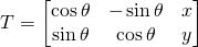
请阅读代码中的注释以进行后续操作。

Python

# Reset stream to first frame 
cap.set(cv2.CAP_PROP_POS_FRAMES, 0) 
 
# Write n_frames-1 transformed frames
for i in range(n_frames-2):
  # Read next frame
  success, frame = cap.read() 
  if not success:
    break
 
  # Extract transformations from the new transformation array
  dx = transforms_smooth[i,0]
  dy = transforms_smooth[i,1]
  da = transforms_smooth[i,2]
 
  # Reconstruct transformation matrix accordingly to new values
  m = np.zeros((2,3), np.float32)
  m[0,0] = np.cos(da)
  m[0,1] = -np.sin(da)
  m[1,0] = np.sin(da)
  m[1,1] = np.cos(da)
  m[0,2] = dx
  m[1,2] = dy
 
  # Apply affine wrapping to the given frame
  frame_stabilized = cv2.warpAffine(frame, m, (w,h))
 
  # Fix border artifacts
  frame_stabilized = fixBorder(frame_stabilized) 
 
  # Write the frame to the file
  frame_out = cv2.hconcat([frame, frame_stabilized])
 
  # If the image is too big, resize it.
  if(frame_out.shape[1] &gt; 1920): 
    frame_out = cv2.resize(frame_out, (frame_out.shape[1]/2, frame_out.shape[0]/2));
  
  cv2.imshow("Before and After", frame_out)
  cv2.waitKey(10)
  out.write(frame_out)

C++

cap.set(CV_CAP_PROP_POS_FRAMES, 1);
Mat T(2,3,CV_64F);
Mat frame, frame_stabilized, frame_out; 
 
 
 
 
for( int i = 0; i &lt; n_frames-1; i++) { bool success = cap.read(frame); if(!success) break; // Extract transform from translation and rotation angle. transforms_smooth[i].getTransform(T); // Apply affine wrapping to the given frame warpAffine(frame, frame_stabilized, T, frame.size()); // Scale image to remove black border artifact fixBorder(frame_stabilized); // Now draw the original and stabilised side by side for coolness hconcat(frame, frame_stabilized, frame_out); // If the image is too big, resize it. if(frame_out.cols &gt; 1920) 
  {
      resize(frame_out, frame_out, Size(frame_out.cols/2, frame_out.rows/2));
  }
 
 
  imshow("Before and After", frame_out);
  out.write(frame_out);
  waitKey(10);
}

步骤5.1:修复边界伪影
当我们稳定一个视频，我们可能会看到一些黑色的边界伪影。这是意料之中的，因为为了稳定视频，帧可能不得不缩小大小。

我们可以通过将视频的中心缩小一小部分(例如4%)来缓解这个问题。

下面的fixBorder函数显示了实现。我们使用getRotationMatrix2D，因为它在不移动图像中心的情况下缩放和旋转图像。我们所需要做的就是调用这个函数时，旋转为0，缩放为1.04(也就是提升4%)。

Python

def fixBorder(frame):
  s = frame.shape
  # Scale the image 4% without moving the center
  T = cv2.getRotationMatrix2D((s[1]/2, s[0]/2), 0, 1.04)
  frame = cv2.warpAffine(frame, T, (s[1], s[0]))
  return frame

C++

void fixBorder(Mat &frame_stabilized)
{
Mat T = getRotationvoid fixBorder(Mat &amp;frame_stabilized)
{
  Mat T = getRotationMatrix2D(Point2f(frame_stabilized.cols/2, frame_stabilized.rows/2), 0, 1.04); 
  warpAffine(frame_stabilized, frame_stabilized, T, frame_stabilized.size()); 
}Matrix2D(Point2f(frame_stabilized.cols/2, frame_stabilized.rows/2), 0, 1.04);
warpAffine(frame_stabilized, frame_stabilized, T, frame_stabilized.size());
}

结果：

我们分享的视频防抖代码的结果如上所示。我们的目标是显著减少运动，但不是完全消除它。

我们留给读者去思考如何修改代码来完全消除帧之间的移动。如果你试图消除所有的相机运动，会有什么副作用?

目前的方法只适用于固定长度的视频，而不适用于实时feed。我们不得不对这个方法进行大量修改，以获得实时视频输出，这超出了本文的范围，但这是可以实现的，更多的信息可以在这里找到。

优点和缺点

优点

这种方法对低频运动(较慢的振动)具有良好的稳定性。这种方法内存消耗低，因此非常适合嵌入式设备(如树莓派)。这种方法对视频缩放抖动有很好的效果。

缺点

这种方法对高频扰动的抵抗效果很差。如果有一个严重的运动模糊，特征跟踪将失败，结果将不是最佳的。这种方法也不适用于滚动快门失真。

代码获取点击源码

爬遍天下无敌手

关注

0
点赞
踩
16

收藏

觉得还不错? 一键收藏
1
评论
OpenCV还能实现这种效果？视频防抖技术！

这篇文章分享了一个视频防抖的策略，这个方法同样可以应用到其他领域，比如常见的关键点检测，当使用视频测试时，效果就没有demo那么好，此时可以考虑本文的方法去优化。分享这些demo并不一定所有人都会用到，但是在解决实际问题的时候，可以提供一个思路去解决问题。希望能给我一个三连，鼓励一下哈在这篇文章中，我们将学习如何使用OpenCV库中的点特征匹配技术来实现一个简单的视频稳定器。我们将讨论算法并且会分享代码(python和C++版)，以使用这种方法在OpenCV中设计一个简单的稳定器。视频中低频.
复制链接

扫一扫