


文章目录
一、作业题目
work with the baseball data set
1)First, filter out all batters with fewer than 100 at bats. Next, standardize all the numerical variables using z-scores.
2)Now, suppose we are interested in estimating the number of home runs, based on the other numerical variables in the data set. So all the other numeric variables will be our predictors. perform PCA
3)How many components should be extracted according to a. The Eigenvalue Criterion? b. The Proportion of Variance Explained Criterion?
3)使用讲过的四种方法确定主成分数目
Use the wine_quality_training data set, available at the textbook web site, for the remaining exercises. The data consist of chemical data about some wines from Portugal. The target variable is quality. Remember to omit the target variable from the dimension-reduction analysis. Unless otherwise indicated, use only the white wines for the analysis
1). Standardize the predictors.
2). Construct a matrix plot of the predictors. Provide a table showing the correlation coefficients of each predictor with each other predictor.
3).apply PCA to the predictors, 使用讲过的四种方法确定主成分数目
baseball和wine
提取码:1234
二、棒球数据集处理
在对数据进行探索之前,要预处理,判断是否有缺失值是必须的:
baseball=read.csv("datasets/baseball.txt",stringsAsFactors=TRUE,sep='')
summary(baseball)
sum(complete.cases(baseball))
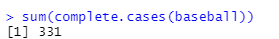
和数据的第一维度相同,故没有缺失值。可以放心做题了。
1.过滤和标准化
(1)实验代码
baseball$age=scale(baseball$age,center = TRUE, scale = TRUE)
baseball[,5:19]=scale(baseball[,5:19],center = TRUE, scale = TRUE)
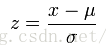
(2)原理介绍
z-score方法如下:
(3)实验结果

(4)结果解释
可以看到上面的数值变量的均值都变成了0.
2.使用PCA
the number of home runs现在是我们的目标变量,其他数值变量都是我们的观测变量,使用PCA试试。
(1)实验代码
# 弄一个新的表
predictor=data.frame(age=baseball$age)
predictor[,2:7]=baseball[,5:10]
predictor[,8:15]=baseball[,12:19]
library(psych)
pca1 <- principal(predictor,nfactors=15,rotate="none", scores=TRUE)
pca1$values
pca1$loadings
(2)实验原理
原理参考我的另一篇博文(如果有耐心看的话)
PCA学习
(3)实验结果

(4)结果解释
可以看到前6个主成分已经包含了92.4%的主要信息。原来的观测变量在每个新的主成分所做出的贡献可以在上面的表中看出,这个表其实就是Y=XP的P矩阵。
3.根据不同判据选取主成分
分别根据下列准则选出主成分:
a. 特征值判据:即拐点
b.主成分特征值累计百分比
c.特征值大于1的主成分
d.根据在各个PCA主成分中的贡献比例筛选原特征
若以a判据:
 如图所示,特征值在5以后基本就平坦了,也就是说取到第4个主成分就可以了。
若以b判据:
以90%为门限,那么根据之前各个特征值得累计比例,可以选择前六个主成分。
若以c判据:
只会选择前四个主成分。
若以d为判据:
loadings(pca1)[,1]^2+loadings(pca1)[,2]^2+loadings(pca1)[,3]^2+loadings(pca1)[,4]^2+
  loadings(pca1)[,5]^2
只选取前5个主成分,结果如下:
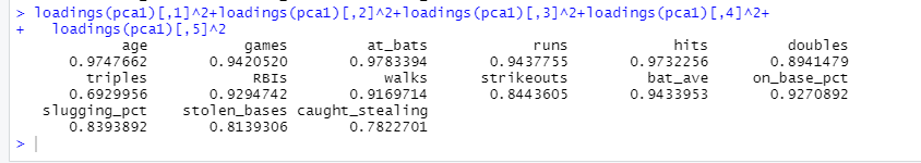 以90%为门限时,保留:age,games,at_bats,runs,hits,RBIS,walks,bat_ave,on_base_pct
三、棒球数据集处理
换了一个数据集,葡萄酒质量数据集。
只是用白葡萄酒的数据。
先进行预处理:
wine=read.csv("datasets/Wine_Quality_Training_File",stringsAsFactors=TRUE,sep='')
head(wine)

- 可以看到很多观测变量是空值,所以我们没有必要留下他们。
- 我们要选用白葡萄酒.
- 体中不涉及目标变量,所以目标变量也不用保留
所以接下来的预处理:
wine=wine[,1:12]
wine=wine[which(wine$type=="white"),]
1.对观测变量进行标准化
(1)实验代码
wine[,2:12]=scale(wine[,2:12],center = TRUE, scale = TRUE)
summary(wine)
(2)原理分析
无
(3)实验结果

(4)结果解释
可以看到上面的数值变量的均值都变成了0.
2.查看各个观测变量之间的线性相关性
(1)实验代码
# 画散点图
pairs(wine[,2:12])
#算相关系数
cor(wine[,2:12])
(2)原理分析
(3)结果展示


(4)结果解释
alcohol和以下特征相关较大:
acid
acid和以下特征相关较大:
sulfur,pH
fixed和以下特征相关较大:
pH
3.使用PCA根据四个判据选主成分
(1)实验代码
library(psych)
pca1 <- principal(wine[,2:12],nfactors=11,rotate="none", scores=TRUE)
pca1$values
pca1$loadings

plot(pca1$values,type = "b",main = "特征值")
loadings(pca1)[,1]^2+loadings(pca1)[,2]^2+loadings(pca1)[,3]^2+loadings(pca1)[,4]^2+
  loadings(pca1)[,5]^2
(2)原理分析
略
(3)实验结果

(4)结果解释
若以a判据:

如图所示,特征值在4以后基本就平坦了,也就是说取到第3个主成分就可以了。
若以b判据:
以90%为门限,那么根据之前各个特征值得累计比例,可以选择前8个主成分。
若以c判据:
只会选择前4个主成分。
若以d为判据:
loadings(pca1)[,1]^2+loadings(pca1)[,2]^2+loadings(pca1)[,3]^2+loadings(pca1)[,4]^2+
  loadings(pca1)[,5]^2
只选取前5个主成分,结果如下:
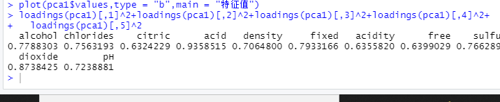
以70%为门限时,保留:alcohol,chlorides,acid,density,fixed,sulfur,dioxide ,pH


 894
894


 被折叠的 条评论
为什么被折叠?
被折叠的 条评论
为什么被折叠?
 到【灌水乐园】发言


