Python计算机视觉编程学习笔记二局部图像描述子

最新推荐文章于 2023-04-25 15:41:28 发布

Belouga-

最新推荐文章于 2023-04-25 15:41:28 发布

阅读量430

点赞数

分类专栏： python 计算机视觉数字图像处理文章标签：计算机视觉 python

本文链接：https://blog.csdn.net/weixin_44330777/article/details/107622442

版权

python 同时被 3 个专栏收录

23 篇文章 1 订阅

订阅专栏

数字图像处理

20 篇文章 10 订阅

订阅专栏

计算机视觉

10 篇文章 0 订阅

订阅专栏

局部图像描述子

本章寻找图像间的对应点和对应区域，介绍用于图像匹配的两种局部描述子算法。图像的局部特征是许多计算机视觉算法的基础，使用特征点来代表图像的内容包括运动目标跟踪，物体识别，图像配准，全景图像拼接，三维重建等。同时由于SIFT算法专利版权所属，本章一些实验做得不是很好，期待后续学习中可以改进。

（一）Harris 角点检测器

1.1 Harris角点检测算法

Harris角点检测算法（也称Harris&Stephens角点检测器）是一个极为简单的交点检测算法。该算法的主要思想是，如果像素周围显示存在多于一个方向的边，我们认为该点为兴趣点。该点就称为角点。

Harris 角点检测算子： Harris 算子是一种简单的点特征提取算子，这种算子受信号处理中自相关函数的启发，给出与自相关函数相联系的矩阵M。M阵的特征值是自相关函数的一阶曲率，如果两个曲率值都高，那么就认为该点是特征点。为了消除噪声对于角点检测的影响，可以使用一个高斯滤波器来平滑图像。
图像域中点x上的对称半正定矩阵 $M I = M I (x)$ 定义为：
在这里插入图片描述
其中 ∆I为包含导数 $I x$ 和 $I y$ 的图像梯度。由于该定义，MIMI 的秩为 1，特征值为 $λ 1 = ∣ ∆ I ∣ 2$ 和 $λ 2 = 0$ 。现在对于图像的每一个像素，我们可以计算出该矩阵。
选择权重矩阵 $W$ （通常为高斯滤波器 $G σ$ ），可以得到卷积:
在这里插入图片描述
该卷积的目的是得到 $M I$ 在周围像素上的局部平均。计算出的矩阵 $M I$ 称为 Harris矩阵。
Harris角点性质：

阈值决定检测点数量：增大α的值，将减小角点响应值R，降低角点检测的灵性，减少被检测角点的数量；减小αα值，将增大角点响应值R，增加角点检测的灵敏性，增加被检测角点的数量。
对亮度和对比度的变化不敏感：由于使用了微分算子对图像进行微分运算，而微分运算对图像密度的拉升或收缩和对亮度的抬高或下降不敏感。
具有旋转不变性：该算子使用的是角点附近的区域灰度二阶矩矩阵。而二阶矩矩阵可以表示成一个椭圆，椭圆的长短轴正是二阶矩矩阵特征值平方根的倒数。当特征椭圆转动时，特征值并不发生变化，所以判断角点响应值也不发生变化，由此说明Harris角点检测算子具有旋转不变性。
不具有尺度不变性。

Harris角点检测中需要用到的函数：

用于计算角点检测器响应函数：

from scipy.ndimage import filters
def compute_harris_response(im,sigma=3):
    #在一幅灰度图像中，再每个像素计算harris角点检测器响应函数
    #计算导数
    imx = zeros(im.shape)
    filters.gaussian_filter(im,(sigma,sigma),(0,1),imx)
    imy = zeros(im.shape)
    filters.gaussian_filter(im,(sigma,sigma),(0,1),imy)
    
    #计算Harris矩阵的分量
    Wxx = filters.gaussian_filter(imx*imx,sigma)
    Wxy = filters.gaussian_filter(imx*imy,sigma)
    Wyy = filters.gaussian_filter(imy*imy,sigma)
    
    #计算特征值和迹
    Wdet = Wxx*Wyy -Wxy**2
    Wtr = Wxx + Wyy
    
    return Wdet/Wtr

用于获取所有的候选像素点和角点响应值递减的顺序排序：

def get_harris_points(harrisim,min_dist=10,threshold=0.1):
    #从一幅harris响应图像中返回角点。min_dist为分割角点和图像边界的最少像素数目 
    #寻找高于阈值的候选角点 
    corner_threshold = harrisim.max()*threshold
    harrisim_t = (harrisim>corner_threshold)*1
    
    #得到候选点的坐标
    coords = array(harrisim_t.nonzero()).T 
    #候选点的Harris响应值
    candidate_values = [harrisim[c[0],c[1]] for c in coords]
    #对候选点按照Harris响应值进行排序
    index = argsort(candidate_values)
    #将可行点的位置保存到数组中
    allowed_locations = zeros(harrisim.shape)
    allowed_locations[min_dist:-min_dist,min_dist:-min_dist] = 1
    #按照min_distance原则，选择最佳harris点
    filtered_coords = []
    for i in index:
        if allowed_locations[coords[i,0],coords[i,1]] == 1:
            filtered_coords.append(coords[i])
            allowed_locations[(coords[i,0]-min_dist):(coords[i,0]+min_dist),
                              (coords[i,1]-min_dist):(coords[i,1]+min_dist)] = 0
    return filtered_coords

显示图像中的角点：

def plot_harris_points(image,filtered_coords):
    #绘制图像中检测到的角点
    figure()
    gray()
    imshow(image)
    plot([p[1] for p in filtered_coords],[p[0] for p in filtered_coords],'*')
    axis('off')
    show()

示例：

from pylab import *
from PIL import Image
from PCV.localdescriptors import harris
# 读入图像
im = array(Image.open('D:\Data\school.jpg').convert('L'))
# 检测harris角点
harrisim = harris.compute_harris_response(im)
# Harris响应函数
harrisim1 = 255 - harrisim
figure()
gray()
#画出Harris响应图
subplot(141)

imshow(harrisim1)
print (harrisim1.shape)
axis('off')
axis('equal')

threshold = [0.01, 0.05, 0.1]
for i, thres in enumerate(threshold):
    filtered_coords = harris.get_harris_points(harrisim, 6, thres)
    subplot(1, 4, i+2)
    imshow(im)
    print (im.shape)
    plot([p[1] for p in filtered_coords], [p[0] for p in filtered_coords], '*')
    axis('off')

#原书采用的PCV中PCV harris模块
#harris.plot_harris_points(im, filtered_coords)

# plot only 200 strongest
# harris.plot_harris_points(im, filtered_coords[:200])

show()

处理效果：
在这里插入图片描述
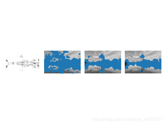
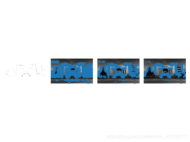
分析：

增大α的值，将减小角点响应值R，降低角点检测的灵性，减少被检测角点的数量；减小α值，将增大角点响应值R，增加角点检测的灵敏性，增加被检测角点的数量。使用阈值 0.01、0.05 和 0.1 检测出的角点依次减少。

1.2 图像中寻找对应点

Harris 角点检测器仅仅能够检测出图像中的兴趣点，但是没有给出通过比较图像间的兴趣点来寻找匹配角点的方法。我们需要在每个点上加入描述子信息，并给出一个比较这些描述子的方法。

兴趣点描述子是分配给兴趣点的一个向量，描述该点附近的图像的表观信息。描述子越好，寻找到的对应点越好。我们用对应点或者点的对应来描述相同物体和场景点在不同图像上形成的像素点。

示例：

from PCV.localdescriptors import harris
from pylab import *
from PIL import Image
im1 = array(Image.open('D:\Data\school.jpg').convert("L"))
im2 = array(Image.open('D:\Data\school.jpg').convert("L"))
wid = 5
harrisim = harris.compute_harris_response(im1, 5)
filtered_coords1 = harris.get_harris_points(harrisim, wid + 1)
d1 = harris.get_descriptors(im1, filtered_coords1, wid)
harrisim = harris.compute_harris_response(im2, 5)
filtered_coords2 = harris.get_harris_points(harrisim, wid + 1)
d2 = harris.get_descriptors(im2, filtered_coords2, wid)
print('starting mathching')
matches = harris.match_twosided(d1, d2)
figure()
gray()
harris.plot_matches(im1, im2, filtered_coords1, filtered_coords2, matches)
show()

处理效果：
在这里插入图片描述

分析：
发现该算法存在一些不正确的匹配，是由于图像像素块的互相关矩阵具有较弱的描述性，在实际运用中，可以使用更加稳健的方法来处理这些对应匹配。但是，总的来说，在要求并不是很高的情况下，这种描述点匹配的方法是最简便的一种处理方法。这些描述符还有一个问题，它们不具有尺度不变性和旋转不变性，而算法中像素块的大小也会影响对应匹配的结果。

（二）SIFT（尺度不变特征变换）

David Lowe提出的SIFT(Scale-Invariant Feature Transform)是最成功的图像局部描述子之一。SIFT特征包括兴趣点检测器和描述子，其中SIFT描述子具有非常强的稳健性，这在很大程度上也是SIFT特征能够成功和流行的主要原因。SIFT特征对于尺度、旋转、亮度都具有不变性，下面会详细介绍其原理。

2.1 尺度空间的构建

图像的尺度空间是这幅图像在不同解析度下的表示。一幅图像可以产生几组（octave）图像，一组图像包括几层图像。构造尺度空间传统的方法即构造一个高斯金字塔，原始图像作为最底层，然后对图像进行高斯模糊再降采样（2倍）作为下一层图像（即尺度越大，图像越模糊），循环迭代下去。
在这里插入图片描述
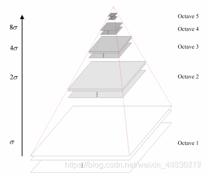
对图像进行尺度变换，以满足特征点的尺度不变性，保留图像轮廓和细节。

2.2 定位兴趣点

SIFT特征使用高斯差分函数来定位兴趣点：

在这里插入图片描述其中， $G σ$ 是二维高斯核， $I σ$ 是使用 $G σ$ 模糊的灰度图像，κ是决定相差尺度的常熟。兴趣点是在图像位置和尺度变换下 $D (x, σ)$ 的最大值和最小值点。这些候选位置通过滤波去除不稳定点。基于一些准则，比如认为低对比度和位于边上的点不是兴趣点，则可以去除一些候选兴趣点。

2.3 描述子

对于上面讨论的兴趣点（关键点）位置描述子给出了兴趣点的位置和尺度信息。为了实现旋转不变性，基于每个点周围图像梯度的方向和大小，SIFT描述子又引入了参考方向。SIFT描述子使用主方向描述参考方向。主方向使用方向直方图（以大小为权重）来度量。

2.4 检测兴趣点

使用开源工具包 VLFeat 提供的二进制文件来计算图像的 SIFT 特征。VLFeat 工具包可以从 http://www.vlfeat.org/ 下载，二进制文件可以在所有主要的平台上运行。

示例：

# -*- coding: utf-8 -*-
from PIL import Image
from pylab import *
from PCV.localdescriptors import sift
from PCV.localdescriptors import harris

# 添加中文字体支持
from matplotlib.font_manager import FontProperties

font = FontProperties(fname=r"c:\windows\fonts\SimSun.ttc", size=14)

imname = 'D:\\Python\\chapter2\\jimei2.jpg'
im = array(Image.open(imname).convert('L'))
sift.process_image(imname, 'empire.sift')
l1, d1 = sift.read_features_from_file('empire.sift')

figure()
gray()
subplot(131)
sift.plot_features(im, l1, circle=False)
title(u'(a)SIFT特征', fontproperties=font)
subplot(132)
sift.plot_features(im, l1, circle=True)
title(u'(b)用圆圈表示SIFT特征尺度', fontproperties=font)

# 检测harris角点
harrisim = harris.compute_harris_response(im)

subplot(133)
filtered_coords = harris.get_harris_points(harrisim, 6, 0.1)
imshow(im)
plot([p[1] for p in filtered_coords], [p[0] for p in filtered_coords], '*')
axis('off')
title(u'(c)Harris角点', fontproperties=font)

show()

处理效果：
在这里插入图片描述
示例2:比较SIFT特征和Harris特征匹配

# -*- coding: utf-8 -*-
from PIL import Image
from pylab import *
from PCV.localdescriptors import sift
from PCV.localdescriptors import harris

# 添加中文字体支持
from matplotlib.font_manager import FontProperties

font = FontProperties(fname=r"c:\windows\fonts\SimSun.ttc", size=14)

imname = 'D:\Data\JiMei.jpg'
im = array(Image.open(imname).convert('L'))
sift.process_image(imname, 'empire.sift')
l1, d1 = sift.read_features_from_file('empire.sift')
figure()
gray()
subplot(131)
sift.plot_features(im, l1, circle=False)
title(u'(a)SIFT特征', fontproperties=font)
subplot(132)
sift.plot_features(im, l1, circle=True)
title(u'(b)用圆圈表示SIFT特征尺度', fontproperties=font)
# 检测harris角点
harrisim = harris.compute_harris_response(im)
subplot(133)
filtered_coords = harris.get_harris_points(harrisim, 6, 0.1)
imshow(im)
plot([p[1] for p in filtered_coords], [p[0] for p in filtered_coords], '*')
axis('off')
title(u'(c)Harris角点', fontproperties=font)
show()

处理效果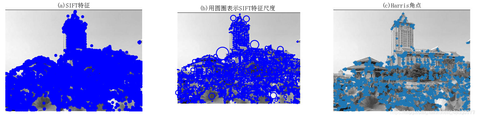：在这里插入图片描述
总结：简单运用sift算法得到如上结果，从中发现，sift算法角点检测和harris角点检测不同，选取的兴趣点也不一样。SIFT选取的对象会使用DoG检测关键点，并且对每个关键点周围的区域计算特征向量，它主要包括两个操作：检测和计算，操作的返回值是关键点信息和描述符，最后在图像上绘制关键点。

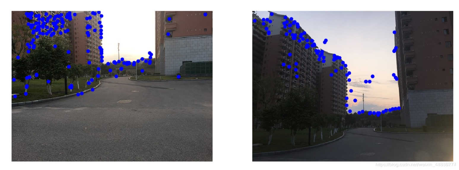
2.5 匹配描述子

对于将一幅图像中的特征匹配到另一幅图像的特征，一种稳健的准则（同样是由 Lowe 提出的）是使用这两个特征距离和两个最匹配特征距离的比率。相比于图像中的其他特征，该准则保证能够找到足够相似的唯一特征。使用该方法可以使错误的匹配数降低。

示例：

from PIL import Image
from pylab import *
import sys
from PCV.localdescriptors import sift

if len(sys.argv) >= 3:
    im1f, im2f = sys.argv[1], sys.argv[2]
else:
    im1f = 'D:\Data\xiaoqu.jpg'
    im2f = 'D:\Data\JiMei.jpg'
im1 = array(Image.open(im1f))
im2 = array(Image.open(im2f))
sift.process_image(im1f, 'out_sift_1.txt')
l1, d1 = sift.read_features_from_file('out_sift_1.txt')
figure()
gray()
subplot(121)
sift.plot_features(im1, l1, circle=False)
sift.process_image(im2f, 'out_sift_2.txt')
l2, d2 = sift.read_features_from_file('out_sift_2.txt')
subplot(122)
sift.plot_features(im2, l2, circle=False)
# matches = sift.match(d1, d2)
matches = sift.match_twosided(d1, d2)
print '{} matches'.format(len(matches.nonzero()[0]))
figure()
gray()
sift.plot_matches(im1, im2, l1, l2, matches, show_below=True)
show()

在这里插入图片描述
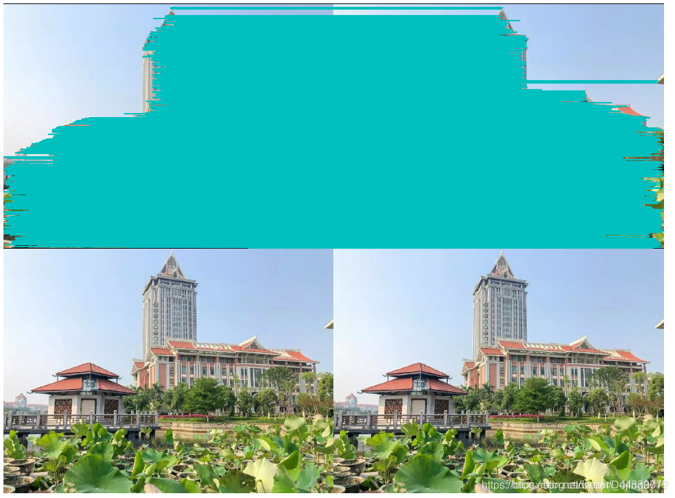
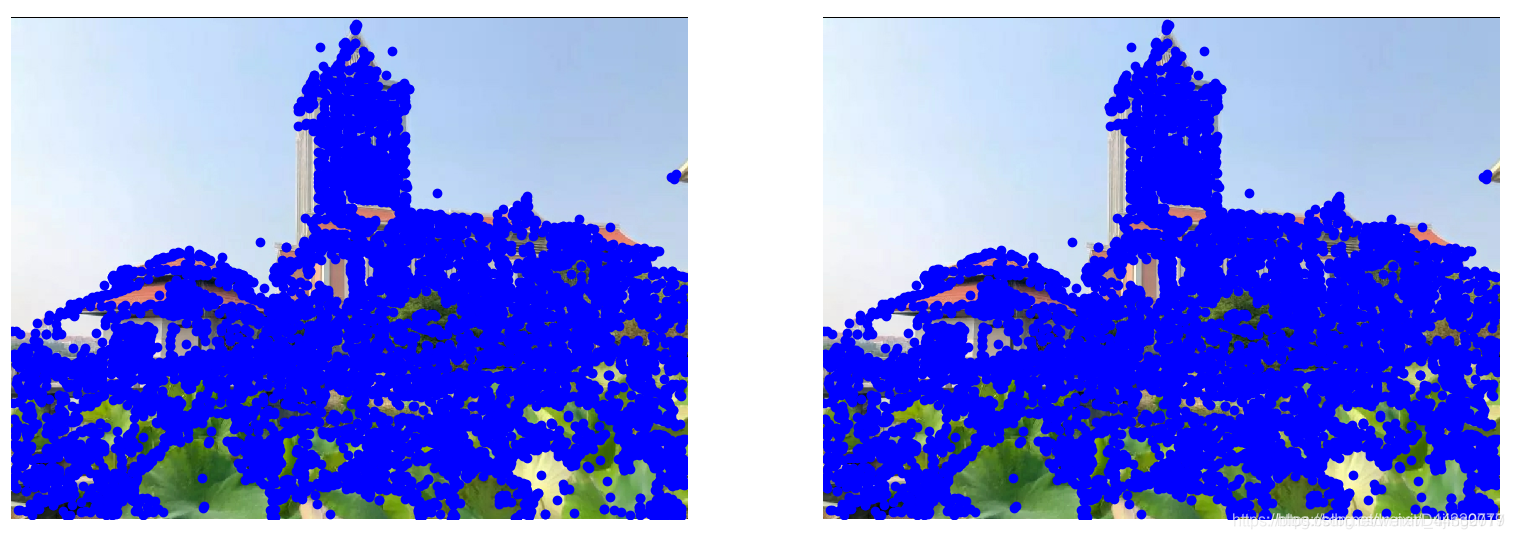
分析：

SIFT算法的实质是在不同的尺度空间上查找关键点(特征点)，并计算出关键点的方向。SIFT所查找到的关键点是一些十分突出，不会因光照，仿射变换和噪音等因素而变化的点，如角点、边缘点、暗区的亮点及亮区的暗点等。

(三) 地理标记图像匹配

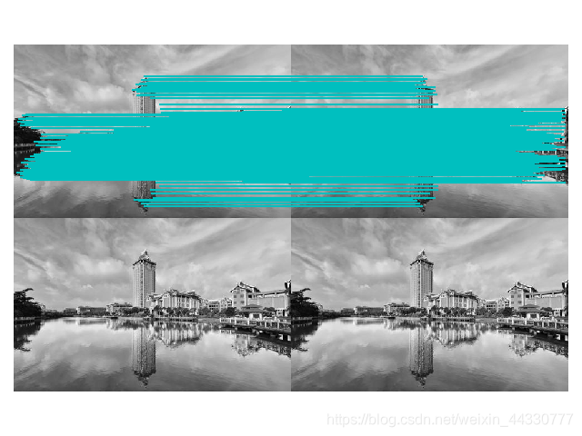
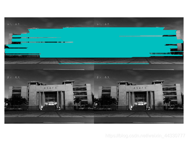
通过不同角度拍摄了照片并进行地理标记图像匹配。
在进行实验前要先安装完GraphViz，否则会出现如下错误：
在这里插入图片描述示例：

#-*- coding: utf-8 -*-
from pylab import *
from PIL import Image
from PCV.localdescriptors import sift
from PCV.tools import imtools
import pydot

download_path = "D:\Data\school\shangdalou"  # set this to the path where you downloaded the panoramio images
path = "D:\Data\school\shangdalou"  # path to save thumbnails (pydot needs the full system path)
#list of downloaded filenames
imlist = imtools.get_imlist(download_path)
nbr_images = len(imlist)
#extract features
featlist = [imname[:-3] + 'sift' for imname in imlist]
for i, imname in enumerate(imlist):
    sift.process_image(imname, featlist[i])

matchscores = zeros((nbr_images, nbr_images))

for i in range(nbr_images):
    for j in range(i, nbr_images):  # only compute upper triangle
        print ('comparing ', imlist[i], imlist[j])
        l1, d1 = sift.read_features_from_file(featlist[i])
        l2, d2 = sift.read_features_from_file(featlist[j])
        matches = sift.match_twosided(d1, d2)
        nbr_matches = sum(matches > 0)
        print ('number of matches = ', nbr_matches)
        matchscores[i, j] = nbr_matches
print ("The match scores is: \n", matchscores)

#copy values
for i in range(nbr_images):
    for j in range(i + 1, nbr_images):  # no need to copy diagonal
        matchscores[j, i] = matchscores[i, j]

#可视化

threshold = 2  # min number of matches needed to create link

g = pydot.Dot(graph_type='graph')  # don't want the default directed graph

for i in range(nbr_images):
    for j in range(i + 1, nbr_images):
        if matchscores[i, j] > threshold:
            # first image in pair
            im = Image.open(imlist[i])
            im.thumbnail((100, 100))
            filename = path + str(i) + '.png'
            im.save(filename)  # need temporary files of the right size
            g.add_node(pydot.Node(str(i), fontcolor='transparent', shape='rectangle', image=filename))

            # second image in pair
            im = Image.open(imlist[j])
            im.thumbnail((100, 100))
            filename = path + str(j) + '.png'
            im.save(filename)  # need temporary files of the right size
            g.add_node(pydot.Node(str(j), fontcolor='transparent', shape='rectangle', image=filename))

            g.add_edge(pydot.Edge(str(i), str(j)))
g.write_png('b.png')

处理效果：
在这里插入图片描述
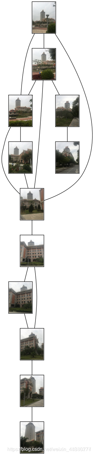
分析：
从这张图可以看出，在遮挡物较多时，图片仅能匹配到图片中的标志性建筑大楼，最终匹配结果图片十分狭长，匹配的最终结果并不很好，一张图出现了重复匹配的现象。可能是图像压缩得太小了，失去了图像原本的特征，导致匹配结果出错。

Belouga-

关注

0
点赞
踩
2

收藏

觉得还不错? 一键收藏
0
评论
Python计算机视觉编程学习笔记二局部图像描述子

寻找图像间的对应点和对应区域。介绍用于图像匹配的两种局部描述子算法。图像的局部特征是许多计算机视觉算法的基础，使用特征点来代表图像的内容包括运动目标跟踪，物体识别，图像配准，全景图像拼接，三维重建等...
复制链接

扫一扫