Python机器学习笔记（一）

前言

监督学习、无监督学习、半监督学习、强化学习

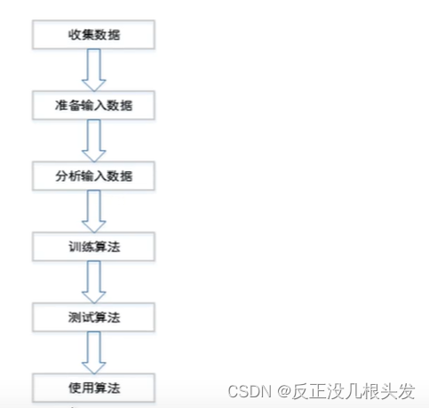
机器学习程序开发步骤

1、Numpy函数库

①numpy.array() 数组

>>> import numpy as np

>>> a = np.array([[1,2,3],[4,5,6]])   # 创建一个二维数组
>>> type(a)
<class 'numpy.ndarray'>

>>> a.shape
(2, 3)

>>> b = np.array([[[1],[2],[3]]])	# 创建一个三维数组
>>> b.shape
(1, 3, 1)
>>> b.shape[1]	# shape返回的是一个元组，可以通过下标访问
3

>>> x = np.random.rand(2,3)	# 生成随机数组
>>> x
array([[0.42630003, 0.30314511, 0.68262633],
       [0.26686761, 0.34573572, 0.97445957]])
>>> x.dtype
dtype('float64')

>>> a.dtype
dtype('int32')
>>> b.dtype
dtype('int32')

数组点乘

numpy.dot(x,y)
或 x.dot(y)

>>> a = np.array([1,2,3])
>>> a
array([1, 2, 3])
>>> b = np.array([4,5,6])
>>> b
array([4, 5, 6])

>>> np.dot(a,b)
32

>>> a.dot(b)
32

>>> np.matmul(a,b)
32

数组数量积 (区别：矩阵数量积是multiply())
*

>>> a = np.array([1,2,3])
>>> a
array([1, 2, 3])
>>> b = np.array([4,5,6])
>>> b
array([4, 5, 6])

>>> a * b
array([ 4, 10, 18])

数组和矩阵

>>> a = np.array([[1,2,3],[4,5,6]])
>>> a
array([[1, 2, 3],
       [4, 5, 6]])
       
>>> a1 = np.matrix('1 2 3;4 5 6')
>>> a1
matrix([[1, 2, 3],
        [4, 5, 6]])

②numpy.matrix() 矩阵

矩阵的创建

>>> import numpy as np

>>> a1 = np.matrix('1 2 3;4 5 6')
>>> a1
matrix([[1, 2, 3],
        [4, 5, 6]])
>>> type(a1)
<class 'numpy.matrix'>
>>> a1.dtype
dtype('int32')

另一种矩阵创建方式：numpy.mat()

>>> b1 = np.mat('1 2 3;4 5 6')
>>> b1
matrix([[1, 2, 3],
        [4, 5, 6]])

mat()中的参数可以是一个数组

>>> x = np.random.rand(2,3)	# 生成随机数组
>>> x
array([[0.42630003, 0.30314511, 0.68262633],
       [0.26686761, 0.34573572, 0.97445957]])
>>> type(x)
<class 'numpy.ndarray'>

>>> x1 = np.mat(x)
>>> x1
matrix([[0.42630003, 0.30314511, 0.68262633],
        [0.26686761, 0.34573572, 0.97445957]])
>>> type(x1)
<class 'numpy.matrix'>

矩阵的转置

a.T 或者 a.transpose()

>>> a1
matrix([[1, 2, 3],
        [4, 5, 6]])
>>> a1.T
matrix([[1, 4],
        [2, 5],
        [3, 6]])
>>> a1.transpose()
matrix([[1, 4],
        [2, 5],
        [3, 6]])

矩阵的乘法

* 或者 np.matmul(a,b)

>>> a1 * a2
matrix([[14, 32],
        [32, 77]])
        
>>> np.matmul(a1,a2)
matrix([[14, 32],
        [32, 77]])

求数量积：对应位置的元素相乘,np.multiply()

>>> c
matrix([[1, 4, 5],
        [7, 5, 1],
        [8, 4, 2]])
>>> np.multiply(c,c)
matrix([[ 1, 16, 25],
        [49, 25,  1],
        [64, 16,  4]])

矩阵求逆

导入numpy.linalg包，使用其中的**inv()**函数

>>> import numpy.linalg as lg
>>> c = np.matrix('1 4 5; 7 5 1;8 4 2')
>>> c
matrix([[1, 4, 5],
        [7, 5, 1],
        [8, 4, 2]])
>>> lg.inv(c)
matrix([[-0.07692308, -0.15384615,  0.26923077],
        [ 0.07692308,  0.48717949, -0.43589744],
        [ 0.15384615, -0.35897436,  0.29487179]])

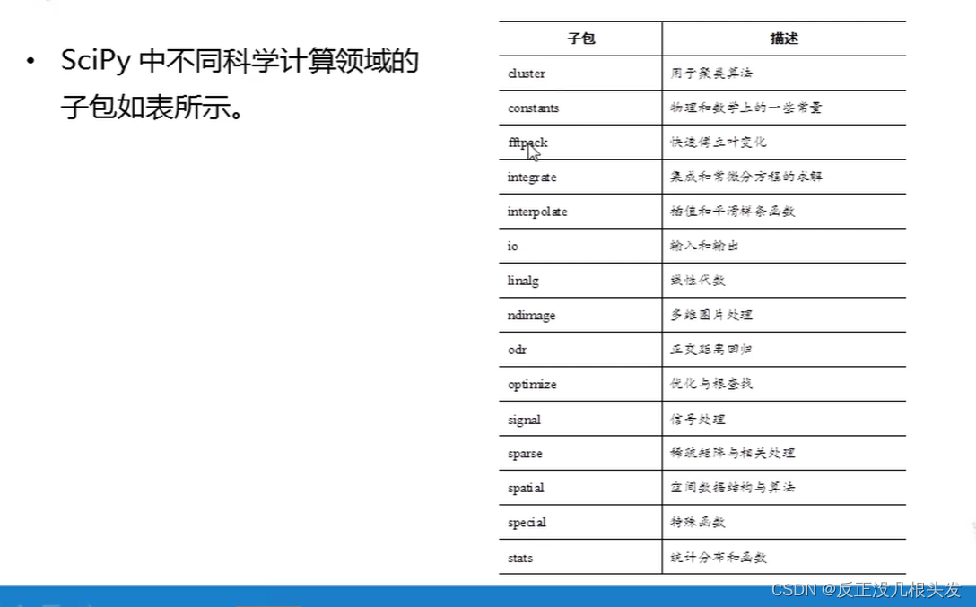
2、Scipy函数库

stats子包

>>> from scipy import stats

norm 正态分布

scipy.stats.norm.cdf(x) 正态函数的分布函数F(x)（累积概率密度函数）

>>> stats.norm.cdf(0)	# 即F(0) = 0.5
0.5
>>> stats.norm.cdf(1)	# 即F(1) = 0.84
0.8413447460685429
>>> stats.norm.cdf([0,1])	# 即F(0) = 0.5、F(1) = 0.84
array([0.5       , 0.84134475])

scipy.stats.norm.rvs(size=?) 生成服从该分布的随机变量，规模为size

>>> stats.norm.rvs(size = 5)
array([-1.89665347,  0.14890029, -0.0892107 ,  1.48550078, -1.61557367])
>>> stats.norm.rvs(size = 2)
array([-1.09398529, -0.02738022])

3、matplotlib库

pyplot子包

from matpltlib import pyplot as plt

绘制坐标

plt.scatter(x轴,y轴)

设置x轴、y轴、图表 名称

plt.xlabel = "x轴名称"
plt.ylabel = "y轴名称"
plt.title = "图表名称"

画2D图像

from numpy import array
from matplotlib import pyplot as plt
from numpy.random import normal

def getData():
    heights = []
    weights = []
    grades = []
    N = 10000
    for i in range(N):
        while True:
            height = normal(172,6)
            if height > 0:break
        while True:
            weight = (height - 80) * 0.7 + normal(0,1)
            if weight > 0:break
        while True:
            score = normal(70,15)
            if 0 < score and score <= 100:
                grade = ('E' if score < 60 else ('D' if score < 70 else ('C' if score < 80 else ('B' if score < 90 else 'A'))))
                break
        heights.append(height)
        weights.append(weight)
        grades.append(grade)
    return array(heights),array(weights),array(grades)

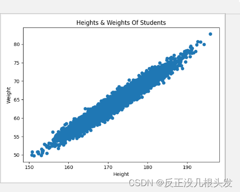
def drawScatter(height,weight):
    plt.scatter(height,weight)
    plt.xlabel("Height")	# x轴坐标
    plt.ylabel("Weight")
    plt.title("Heights & Weights Of Students")
    plt.show()

data = getData()
heights = data[0]
weights = data[1]
drawScatter(heights,weights)

np.meshgrid()

X, Y = np.meshgrid(x, y) 代表的是将x中每一个数据和y中每一个数据组合生成很多点,然后将这些点的x坐标放入到X中,y坐标放入Y中,并且相应位置是对应的，解释如下：

如: x = [1, 2, 3, 4]
    y = [7, 8, 9]
   
x和y中的每一个元素组合生成
[[[1, 7], [2, 7], [3, 7], [4, 7]],
 [[1, 8], [2, 8], [3, 8], [4, 8]],
 [[1, 9], [2, 9], [3, 9], [4, 9]]]
 
然后
再分别放入X和Y中
X = [[1, 2, 3, 4],
	 [1, 2, 3, 4],
	 [1, 2, 3, 4]]

Y = [[7, 7, 7, 7],
	 [8, 8, 8, 8],
	 [9, 9, 9, 9],]

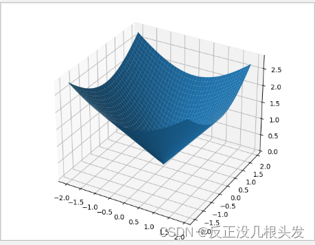
画3D图像

import matplotlib.pyplot as plt
from mpl_toolkits.mplot3d import Axes3D

import numpy as np
import matplotlib.pyplot as plt
from mpl_toolkits.mplot3d import Axes3D

# 创建3D图形数据
fig = plt.figure()
ax = Axes3D(fig)
# 生成数据
X = np.arange(-2,2,0.1)
Y = np.arange(-2,2,0.1)
X,Y = np.meshgrid(X,Y)
Z = np.sqrt(X ** 2 + Y ** 2)
ax.plot_surface(X,Y,Z)
plt.show()