图像质量评价指标

峰值信噪比（Peak Signal-to-Noise Ratio，PSNR）

• PSNR值越大，说明图像信噪比越高，图像的质量就越好。
  给定一个大小为m x n的干净图像I 和噪声图像K，均方误差(MSE)定义为：
  $$MSE=\frac{1}{mn}\sum _{i=0}^{m-1}\sum _{j=0}^{n-1}[I(i,j)-K(i,j){]}^2$$
  然后PSNR(dB)就定义为:
  $$PSNR=10\cdot lo{g}_{10}(\frac{MA{X}_I^2}{MSE})$$
  其中$MA{X}_I^2$为图片可能的最大像素值。
• 如果每个像素值都由8位二进制来表示，那么就为255。
• 通常，如果像素值由B位二进制来表示，那么$MA{X}_I^2$ = $2^B-1$。
  一般地，针对 uint8 数据，最大像素值为 255,；针对浮点型数据，最大像素值为 1。

PSNR代码实现

import torch
from math import log10

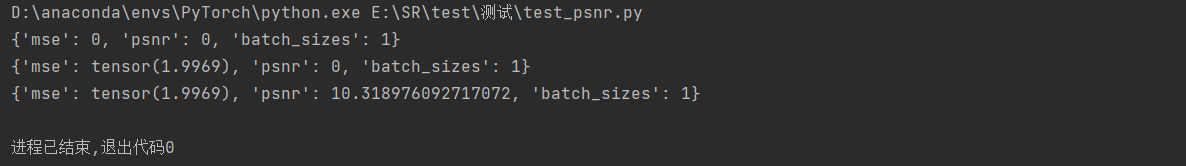
valing_results = {'mse': 0, 'psnr': 0,  'batch_sizes': 0}
sr = torch.randn(1, 3, 339, 339)
hr = torch.randn(1, 3, 339, 339)

batch_size = sr.size(0)  # 1
valing_results['batch_sizes'] += batch_size  # {'mse': 0, 'psnr': 0, 'batch_sizes': 1}
print(valing_results)

batch_mse = ((sr - hr)**2).data.mean()  # tensor(1.9938)
valing_results['mse'] += batch_mse * batch_size  # {'mse': tensor(2.0075), 'psnr': 0, 'batch_sizes': 1}
print(valing_results)

psnr = 10 * log10((hr.max()**2) / (valing_results['mse'] / valing_results['batch_sizes']))
valing_results['psnr'] += psnr
print(valing_results)  # {'mse': tensor(1.9995), 'psnr': 9.678062556486728, 'batch_sizes': 1}

结构相似性（Structural SIMilarity，SSIM）

• SSIM的值域为[0, 1]，值越大说明图像失真越小，两幅图像越相似。
  SSIM公式基于样本x和y之间的三个比较衡量：亮度(luminance)、对比度(contrast)和结构(structure)。
  $$亮度：l(x,y)=\frac{2{\mu }_x{\mu }_y+c_1}{{\mu }_x^2+{\mu }_y^2+c_1}$$$$对比度：c(x,y)=\frac{2{\sigma }_x{\sigma }_y+c_2}{{\sigma }_x^2+{\sigma }_y^2+c_2}$$$$结构：s(x,y)=\frac{{\sigma }_{xy}+c_3}{{\sigma }_x{\sigma }_y+c_3}，一般取c_3=c_2/2，即：s(x,y)=\frac{2{\sigma }_{xy}+c_2}{2{\sigma }_x{\sigma }_y+c_2}$$
  其中：
• ${\mu }_x$：x的均值、${\mu }_y$：y的均值。
• ${\sigma }_x$： x的方差、${\sigma }_y$： y的方差、${\sigma }_{xy}$： xy的协方差。
• $c_1=(K_{1}L{)}^2、c_2=(K_{2}L{)}^2$为两个常数，避免除零。
• $L$：像素值的范围（$2^B-1$）
• $K_1=0.01,K_2=0.03$：默认值
  那么：
  $$SSIM(x,y)=[l(x,y{)}^{\alpha }\cdot c(x,y{)}^{\beta }\cdot s(x,y{)}^{\gamma }]$$
  将$\alpha 、\beta 、\gamma$设为1，可以得到：
  $$SSIM(x,y)=\frac{(2{\mu }_x{\mu }_y+c_1)(2{\sigma }_{xy}+c_2)}{({\mu }_x^2+{\mu }_y^2+c_1)({\sigma }_x^2+{\sigma }_y^2+c_2)}$$
  每次计算的时候都从图片上取一个$N\ast N$的窗口，然后不断滑动窗口进行计算，最后取平均值作为全局的 SSIM。

SSIM代码实现

from math import exp

import torch
import torch.nn.functional as F
from torch.autograd import Variable


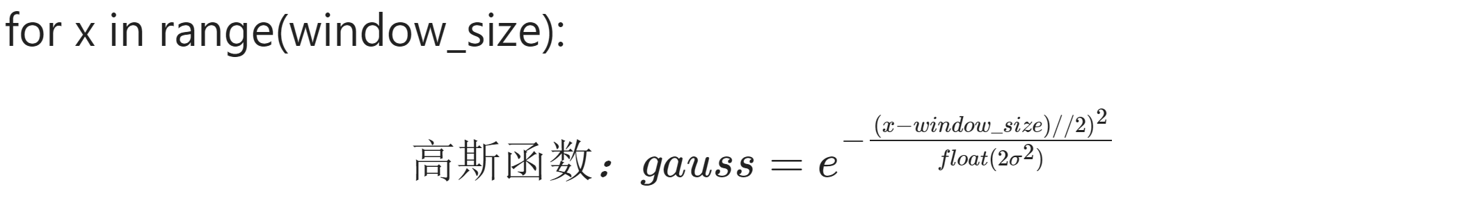
def gaussian(window_size, sigma):
    """
    生成一维高斯滤波函数
    :param window_size: 高斯滤波器的大小
    :param sigma: 高斯函数的标准差
    :return:将计算得到的高斯函数的张量归一化，即将每个元素除以所有元素之和，以确保滤波器的权重总和为1，然后将归一化后的结果作为函数的返回值
    """
    # 对于每个x在range(window_size)范围内，都计算了高斯函数的值
    gauss = torch.Tensor([exp(-(x - window_size // 2) ** 2 / float(2 * sigma ** 2)) for x in range(window_size)])  # [11]
    return gauss / gauss.sum()


def create_window(window_size, channel):
    """创建高斯核（二维窗口）
    .unsqueeze(): （仅改变形状）
    .expand(): （复制指定维度次数的数据，到新的形状）"""
    # 生成一个一维的高斯滤波器：.unsqueeze(1):（仅改变形状） 在第二维度上增加一个维度 [11] --> [11, 1]
    _1D_window = gaussian(window_size, 1.5).unsqueeze(1)  # [11, 1]
    # 将 _1D_window 与其转置相乘，生成一个二维的高斯滤波器 [11, 1]*[1, 11]=[11, 11]  --> [1, 1, 11, 11]
    _2D_window = _1D_window.mm(_1D_window.t()).float().unsqueeze(0).unsqueeze(0)  # [1, 1, 11, 11]
    # 将 _2D_window 在第一个维度上进行扩展，以适应输入数据的通道数 .expend():将数据在第一个维度复制三次 [1, 1, 11, 11] -->[3, 1, 11, 11]
    # .contiguous()：深拷贝：使用expand()改变window的数据内容，对于原始的_2D_window数据没有影响 # 如果不使用的话，——2D——window的数据也会改变
    # https://blog.csdn.net/kdongyi/article/details/108180250
    # Variable(张量, 梯度)：用来包装Tensor，将Tensor转换为Variable之后，可以装载梯度信息。用于方向传播自动计算梯度
    window = Variable(_2D_window.expand(channel, 1, window_size, window_size).contiguous())  # [3, 1, 11, 11]
    return window  # [channel, 1, window_size, window_size]


def _ssim(img1, img2, window, window_size, channel, size_average=True):
    """
    结构相似度：用于比较两幅图像的相似度
    :param img1: sr[1, 3, 1356, 1356]
    :param img2: hr[1, 3, 1356, 1356]
    :param window: 卷积核 [3, 1, 11, 11]
    :param window_size: 11
    :param channel: 3
    :param size_average: True
    :return:
    """
    # 均值
    # F.conv2d([1, 3, 1356, 1356], [3, 1, 11, 11], 5, 3)：1个3通道的1356*1356图像与3个单通道的11*11卷积核进行groups=3的逐层卷积运算
    # 注意卷积核的个数必须是输入数据通道数的整数倍， 且输出数据的通道数与卷积核的个数一致
    mu1 = F.conv2d(img1, window, padding=window_size // 2, groups=channel)  # [1, 3, 1356, 1356]
    mu2 = F.conv2d(img2, window, padding=window_size // 2, groups=channel)  # [1, 3, 1356, 1356]

    # 平方
    mu1_sq = mu1.pow(2)
    mu2_sq = mu2.pow(2)
    mu1_mu2 = mu1 * mu2

    # 方差图像：分通道计算输入图像的平方与均值图像平方的差异
    sigma1_sq = F.conv2d(img1 * img1, window, padding=window_size // 2, groups=channel) - mu1_sq  # [1, 3, 1356, 1356]
    sigma2_sq = F.conv2d(img2 * img2, window, padding=window_size // 2, groups=channel) - mu2_sq  # [1, 3, 1356, 1356]

    # 协方差图像：计算输入图像乘积与均值图像乘积的差异
    sigma12 = F.conv2d(img1 * img2, window, padding=window_size // 2, groups=channel) - mu1_mu2  # [1, 3, 1356, 1356]

    C1 = 0.01 ** 2  # (0.01)^2= 0.0001
    C2 = 0.03 ** 2  # (0.03)^2=0.0009

    # ssim_map = ((2 * a*b +  c1) * (2 * 协方差 + C2)) / (a^2 + b^2 + C1) * (a方差 + b方差 + C2 )
    ssim_map = ((2 * mu1_mu2 + C1) * (2 * sigma12 + C2)) / ((mu1_sq + mu2_sq + C1) * (sigma1_sq + sigma2_sq + C2))  # [1, 3, 1356, 1356]

    if size_average:
        return ssim_map.mean()
    else:
        return ssim_map.mean(1).mean(1).mean(1)


class SSIM(torch.nn.Module):
    def __init__(self, window_size=11, size_average=True):
        super(SSIM, self).__init__()
        self.window_size = window_size
        self.size_average = size_average
        self.channel = 1
        self.window = create_window(window_size, self.channel)  # [channel, 1, window_size, window_size]

    def forward(self, img1, img2):
        (_, channel, _, _) = img1.size()

        # 如果图像的通道数与保存的通道数相同，并且窗口数据类型与图像的数据类型相同，就直接使用保存的窗口；
        # 否则，重新创建窗口，并根据图像是否在 GPU 上进行相应的处理。
        if channel == self.channel and self.window.data.type() == img1.data.type():
            window = self.window
        else:
            window = create_window(self.window_size, channel)

            if img1.is_cuda:
                window = window.cuda(img1.get_device())
            window = window.type_as(img1)  # b = type_as(a): 将b的数据类型变成跟a一样的类型

            self.window = window
            self.channel = channel

        return _ssim(img1, img2, window, self.window_size, channel, self.size_average)


def ssim(img1, img2, window_size=11, size_average=True):
    (_, channel, _, _) = img1.size()
    window = create_window(window_size, channel)  # [3, 1, 11, 11]

    if img1.is_cuda:
        window = window.cuda(img1.get_device())
    window = window.type_as(img1)

    return _ssim(img1, img2, window, window_size, channel, size_average)

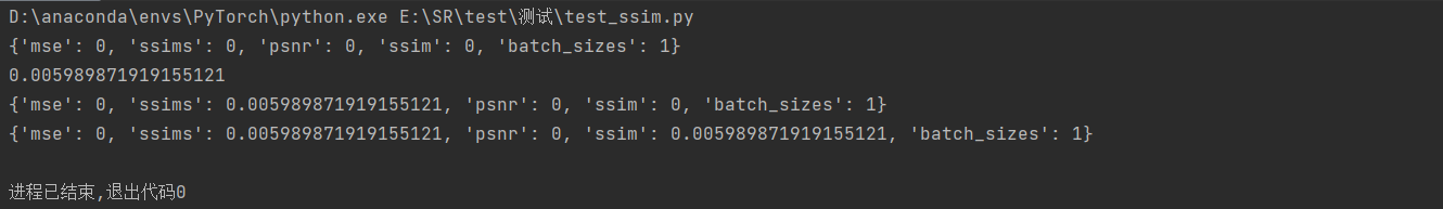
valing_results = {'mse': 0, 'ssims': 0, 'psnr': 0, 'ssim': 0, 'batch_sizes': 0}
sr = torch.randn(1, 3, 1356, 1356)
hr = torch.randn(1, 3, 1356, 1356)

# 计算并保存batch_size
batch_size = sr.size(0)  # 1
valing_results['batch_sizes'] += batch_size  # {'mse': 0, 'psnr': 0, 'batch_sizes': 1}
print(valing_results)

# 计算一个bath的ssim
batch_ssim = ssim(sr, hr).item()
print(batch_ssim)

# 计算并保存所有batch的ssim
valing_results['ssims'] += batch_ssim * batch_size
print(valing_results)

# 计算并保存每个batch_size的ssim
valing_results['ssim'] = valing_results['ssims'] / valing_results['batch_sizes']  # 每个batch的ssim
print(valing_results)

自然图像质量评价器（Natural Image Quality Evaluator，NIQE）

  在进行图像重建任务后通常还要做图像质量评价，常用的判断指标有峰值信噪比(PSNR)，结构相似性(SSIM) 等。在大部分任务中，通过这些指标可以证明图像重建任务是否更加有效。但在超分辨重建任务里，在近些年引入生成对抗网络后，人们发现高的PSNR或SSIM不一定能代表更好重建质量，因为在高PSNR或SSIM的图片中，它们图像的纹理细节并不一定符合人眼的视觉习惯。因此，研究者们找到了这种更有效的图像重建质量的指标NIQE。

  NIQE基于一组“质量感知”特征，并将其拟合到MVG模型中。质量感知特征源于一个简单但高度正则化的NSS模型。然后，将给定的测试图像的NIQE指标表示为从测试图像中提取的NSS特征的MVG模型与从自然图像语料中提取的质量感知特征的MVG模型之间的距离。整个过程由五步操作完成：

1. 空间域NSS（Natural Scene Statistic）
   使用经典的空域NSS模型，对图像进行预处理：
   $$\hat{T}(i,j)=\frac{I(i,j)-\mu (i,j)}{\sigma (i,j)+1}(1)$$

• 其中:
• i ∈ { 1 , 2 , . . . , M } , j ∈ { 1 , 2 , . . . , N } i \in \{1, 2, ..., M\}, j\in \{1, 2, ..., N\} i∈{1,2,...,M},j∈{1,2,...,N}为图像的空间坐标，M与N为图像的空间维度。
• $\mu (i,j)为平滑后的均值图像，\sigma (i,j)为标准差图像$，且：
  $$\mu (i,j)=\sum _{k=-K}^K\sum _{l=-L}^L{\omega }_{k,l}I(i+k,j+l)(2)$$
  $$\sigma (i,j)=\sqrt{\sum _{k=-K}^K\sum _{l=-L}^L{\omega }_{k,l}[I(i,j)-\mu (i,j){]}^2}(3)$$
  • 其中， { ω k , l ∣ k = − K , . . . , K ; l = − L , . . . , L } \{\omega_{k ,l}|k =-K, ..., K;l = -L, ...,L\} {ωk,l​∣k=−K,...,K;l=−L,...,L}是一个从3个标准差(K = L = 3)中采样并重新缩放到单位体积的二维循环对称高斯权函数

2. 图像块（patch）选取
   \quad 一旦计算出公式（1）中的图像系数，图像就会被分割成P×P的patch。然后根据每个patch的系数计算出特定的NSS特征。==方差(3)在之前的基于NSS的图片分析中很大程度上被忽视。但是它在结构化图片信息上有丰富的内容。这些内容可以被用来量化局部图片的锐利度。(从美学上认为一幅图片越锐利它的成像效果会越好，平滑模糊代表一种视觉信息的潜在损失。）==将P×P的图像块用$b=1,2,...,B$做标记，再用一种直接的方法计算每一块b的平均局部偏移范围：
   $$\delta (b)=\sum \sum {}_{(i,j)\in patchb}\sigma (i,j)(4)$$

• 其中, $\delta$表示局部活跃（锐利）度。
  \quad 在求得每块的锐利度后，超过门限 T 的 $\delta$ 将被选中(即：δ>T)。门限 T由块的峰值锐利度 p得到，在原文中p = 0.75 , 作者观察 p在一个小范围[ 0.6 , 0.9] 变化。

3. 特征化图像块
   \quad 给定如上所述选择的自然图像patch的集合，其统计数据的特征是根据每个选定的patch计算的“质量感知”NSS 特征。先前对基于 NSS 的图像质量的研究表明，广义高斯分布有效地捕捉了它们的自然图像和失真图像系数 (1) 的联系。

• 均值为0的广义高斯分布（GGD）公式为：
  $$f(x;\alpha ,\beta )=\frac{\alpha }{2\beta \Gamma (1/\alpha )}exp(-(\frac{|x|}{\beta }{)}^{\alpha })(5)$$
• 其中
• $\Gamma (\cdot )$为伽马函数：$$\Gamma (a)={\int }_0^{\infty }{t}^{a-1}{e}^{-t}dt(a>0)(6)$$
• GGD的参数$(\alpha ,\beta )$可以使用一种moment-matching(矩阵匹配)方法估计出。

推导见原论文：
Estimation of shape parameter for generalized Gaussian distributions in subband decompositions of video

然后，可以用一个均值为0的对称广义高斯分布(AGGD)将领域系数的乘积很好的建模：
$$f(x;\gamma ,{\beta }_l,{\beta }_r)=\{\begin{array}{l}\frac{\gamma }{{\beta }_l+{\beta }_r\Gamma (1/\gamma )exp(-(\frac{-x}{\beta }{)}^{\gamma }}(\forall x\le 0)\\ \frac{\gamma }{{\beta }_l+{\beta }_r\Gamma (1/\gamma )exp(-(\frac{x}{\beta }{)}^{\gamma }}(\forall x\ge 0)\end{array}(7)$$

• 其中，AGGD的参数$(\gamma ,{\beta }_l,{\beta }_r)$ 可以被计算出来，

详细推导见原论文：
Multiscale skewed heavy tailed model for texture analysis

具体计算过程如下：

计算参数${\beta }_l,{\beta }_r$的公式为： $${\hat{\beta }}_l=\sqrt{\frac{1}{N_l-1}\sum _{k=1,x_k<0}^{N_l}{x}_k^2}\times \sqrt{\frac{\Gamma (3/\hat{a})}{\Gamma (1/\hat{a})}}$$ $${\hat{\beta }}_r=\sqrt{\frac{1}{N_r-1}\sum _{k=1,x_k\ge 0}^{N_r}{x}_k^2}\times \sqrt{\frac{\Gamma (3/\hat{a})}{\Gamma (1/\hat{a})}}$$ 其中：

• $\sqrt{\frac{1}{N_l-1}{\sum }_{k=1,x_k<0}^{N_l}{x}_k^2}$ 为图像块中小于0的值的标准差
• $\sqrt{\frac{1}{N_r-1}{\sum }_{k=1,x_k\ge 0}^{N_r}{x}_k^2}$ 为图像块中大于等于0的值的标准差
• 而$\hat{\alpha }$ 的计算公式如下： $$\hat{\alpha }=(r(\gamma )-\hat{r}\frac{({\hat{\gamma }}^3+1)(\hat{\gamma }+1)}{(\hat{\gamma }+1{)}^2}{)}^2$$
  • 其中，$r(\gamma )$为(generalized Gaussian ratio function)广义高斯比率函数:$$r(\gamma )=\frac{\Gamma (2/\gamma {)}^2}{\Gamma (1/\gamma )\Gamma (3/\gamma )}$$
  • $\gamma$是形状参数，从0.2到10.001，步幅为0.001。
  • $\hat{r}$为无偏估计：$$\hat{r}=\frac{(\sum |x_k|{)}^2}{\sum x_k^2}$$
  • $\hat{\gamma }$: $$\hat{\gamma }=\frac{\sqrt{\frac{1}{N_l-1}{\sum }_{k=1,x_k<0}^{N_l}{x}_k^2}}{\sqrt{\frac{1}{N_r-1}{\sum }_{k=1,x_k\ge 0}^{N_r}{x}_k^2}}$$

此外，图像块的特征除了$(\gamma ,{\beta }_l,{\beta }_r)$，特征分布的均值$\eta$ 也很有用：
$$\eta =({\beta }_l-{\beta }_r)\frac{\Gamma (2/\gamma )}{\Gamma (1/\gamma )}(8)$$

4. 多尺度高斯模型（Multivariate Gaussian Model，MVG）
   \quad 通过将自然图像块patches与 MVG 密度函数进行拟合，可以获得一个简单的 NSS 特征模型，从而提供它们的丰富表示，MVG密度函数如下：
   $$f_X(x_1,...,x_k)=\frac{1}{(2\pi {)}^{k/2}|\sum {|}^{1/2}}exp(-\frac{1}{2}(x-v{)}^T(x-v))(9)$$

• 其中:
• $(x_1,...,x_k)$是公式(5)~(8)中计算出的NSS特征$(\gamma ,\eta ,{\beta }_l,{\beta }_r)$。
• $v和\sum$是MVG 模型的均值和协方差矩阵。

5. NIQE指标

  NIQE的计算流程：从要进行质量分析的图像中选取相同P×P大小的patches中计算 36 个相同的 NSS 特征，接着将他们与 MVG 模型进行拟合，然后将其 MVG 拟合模型与自然 MVG 模型进行比较。
（总结：用失真图像的MVG模型与自然语料库中自然图像的MVG模型相比较）

失真图像的质量表示为质量感知 NSS 特征模型和==拟合从失真图像中提取的特征的 MVG ==之间的距离，表达式为：
$$D(v_1,v_2,\sum {}_1,\sum {}_2)=\sqrt{((v_1-v_2{)}^T(\frac{\sum {}_1+\sum 2}{2}{)}^{-1}(v_1-v_2))}(10)$$
其中：

• $v_1,v_2和\sum {}_1,\sum {}_2$是自然 MVG 模型和失真图像 MVG 模型的均值向量和协方差矩阵。

NIQE代码实现

这里使用basicsr中的niqe代码实现，

import cv2
import math
import numpy as np
import os
from scipy.ndimage import convolve  # 数组与给定的内核作卷积运算
from scipy.special import gamma  # 伽马函数

from basicsr.metrics.metric_util import reorder_image, to_y_channel
from basicsr.utils.matlab_functions import imresize
from basicsr.utils.registry import METRIC_REGISTRY

# 中文链接：https://blog.csdn.net/qq_30124657/article/details/114268329


def estimate_aggd_param(block):
    """Estimate AGGD (Asymmetric Generalized Gaussian Distribution) parameters.
    (评估AGGD:非对称广义高斯分布参数)

    Args:
        block (ndarray): 2D Image block.

    Returns:
        tuple: alpha (float), beta_l (float) and beta_r (float) for the AGGD
            distribution (Estimating the parames in Equation 7 in the paper).
    """
    block = block.flatten()  # 将2D图像展平成1维数组
    gam = np.arange(0.2, 10.001, 0.001)  # len = 9801，gam用于参数估计
    gam_reciprocal = np.reciprocal(gam)  # 计算gam数组中每个元素的倒数
    r_gam = np.square(gamma(gam_reciprocal * 2)) / (gamma(gam_reciprocal) * gamma(gam_reciprocal * 3))  # r(r) = T(2/a)^2/[T(1/a)T(3/a)]

    left_std = np.sqrt(np.mean(block[block < 0]**2))  # 计算图像块中小于0的值的标准差
    right_std = np.sqrt(np.mean(block[block > 0]**2))  # 计算图像块中大于0的值的标准差
    gammahat = left_std / right_std
    rhat = (np.mean(np.abs(block)))**2 / np.mean(block**2)  # 图像块绝对值的均值的平方与图像块值的均值的比值。
    rhatnorm = (rhat * (gammahat**3 + 1) * (gammahat + 1)) / ((gammahat**2 + 1)**2)  # r = r_hat *(r^3 +1)(r+1) / (r^2 +1)^2
    array_position = np.argmin((r_gam - rhatnorm)**2)  # 找到使得r_gam和rhatnorm的平方差最小的索引位置。 min((r(r)-r)^2)

    alpha = gam[array_position]  # 根据前一步找到的索引位置，从gam数组中取出对应的alpha值。
    beta_l = left_std * np.sqrt(gamma(1 / alpha) / gamma(3 / alpha))  # 计算beta_l，基于alpha和左侧标准差的一些复杂计算。
    beta_r = right_std * np.sqrt(gamma(1 / alpha) / gamma(3 / alpha))  # 计算beta_r，基于alpha和右侧标准差的一些复杂计算。
    return (alpha, beta_l, beta_r)


def compute_feature(block):
    """Compute features.
    计算当前块的特征

    Args:
        block (ndarray): 2D Image block.

    Returns:
        list: Features with length of 18.
    """
    feat = []
    alpha, beta_l, beta_r = estimate_aggd_param(block)
    feat.extend([alpha, (beta_l + beta_r) / 2])

    # distortions disturb the fairly regular structure of natural images.
    # This deviation can be captured by analyzing the sample distribution of
    # the products of pairs of adjacent coefficients computed along
    # horizontal, vertical and diagonal orientations.
    # 扭曲扰乱了自然图像的相当规则的结构。
    # 这种偏差可以通过分析沿水平、垂直和对角线方向计算的相邻系数对的乘积的样本分布来捕获。
    shifts = [[0, 1], [1, 0], [1, 1], [1, -1]]
    for i in range(len(shifts)):
        shifted_block = np.roll(block, shifts[i], axis=(0, 1))  # : 将图像块按照当前平移偏移在水平和垂直方向进行滚动，得到一个平移后的图像块。
        alpha, beta_l, beta_r = estimate_aggd_param(block * shifted_block)  # 计算当前平移后的图像块与原始图像块的乘积的AGGD分布参数
        # Eq. 8
        mean = (beta_r - beta_l) * (gamma(2 / alpha) / gamma(1 / alpha))
        feat.extend([alpha, mean, beta_l, beta_r])
    return feat


def niqe(img, mu_pris_param, cov_pris_param, gaussian_window, block_size_h=96, block_size_w=96):
    """Calculate NIQE (Natural Image Quality Evaluator) metric.

    ``Paper: Making a "Completely Blind" Image Quality Analyzer``

    This implementation could produce almost the same results as the official
    MATLAB codes: http://live.ece.utexas.edu/research/quality/niqe_release.zip

    Note that we do not include block overlap height and width, since they are
    always 0 in the official implementation.

    For good performance, it is advisable by the official implementation to
    divide the distorted image in to the same size patched as used for the
    construction of multivariate Gaussian model.
    为了获得良好的性能, 官方实现建议将扭曲图像划分为与构建多元高斯模型相同大小的patch

    Args:
        img (ndarray): Input image whose quality needs to be computed. The
            image must be a gray or Y (of YCbCr) image with shape (h, w).
            Range [0, 255] with float type.
        (输入图像的形状必须为 (h, w) 的灰色或 Y(YCbCr)图像。范围 [0, 255] 带浮点型。)

        mu_pris_param (ndarray): Mean of a pre-defined multivariate Gaussian
            model calculated on the pristine dataset.
        (均值：在原始数据集上计算的预定义多元高斯模型的均值)

        cov_pris_param (ndarray): Covariance of a pre-defined multivariate
            Gaussian model calculated on the pristine dataset.
        (协方差：在原始数据集上计算的预定义多元高斯模型的协方差。)

        gaussian_window (ndarray): A 7x7 Gaussian window used for smoothing the
            image.
        (用于平滑图像的 7x7 高斯窗口。)

        block_size_h (int): Height of the blocks in to which image is divided.
            Default: 96 (the official recommended value).
        (图像被分割到的块的高度。默认值:96(官方建议值))

        block_size_w (int): Width of the blocks in to which image is divided.
            Default: 96 (the official recommended value).
        (图像被分割到的块的宽度。默认值: 96(官方推荐值))
    """
    # 确保输入的图像是灰度图或YCbCr格式的图像，并且是二维的（即没有通道维度）。
    assert img.ndim == 2, 'Input image must be a gray or Y (of YCbCr) image with shape (h, w).'
    # crop image
    h, w = img.shape
    num_block_h = math.floor(h / block_size_h)  # 计算patch的数量
    num_block_w = math.floor(w / block_size_w)
    img = img[0:num_block_h * block_size_h, 0:num_block_w * block_size_w]  # 将图像剪裁成patch的整数倍

    distparam = []  # dist param is actually the multiscale features （存储多尺度特征）
    for scale in (1, 2):  # perform on two scales (1, 2)
        mu = convolve(img, gaussian_window, mode='nearest')  # 使用卷积操作对图像进行平滑处理，得到均值图像mu
        sigma = np.sqrt(np.abs(convolve(np.square(img), gaussian_window, mode='nearest') - np.square(mu)))  # 计算标准差图像sigma，用于归一化处理

        # normalize, as in Eq. 1 in the paper  对图像进行归一化处理，得到归一化图像
        img_nomalized = (img - mu) / (sigma + 1)

        feat = []  # 用于存储特征
        for idx_w in range(num_block_w):
            for idx_h in range(num_block_h):
                # process each block
                # 获取当前块的归一化图像
                block = img_nomalized[idx_h * block_size_h // scale:(idx_h + 1) * block_size_h // scale,
                                      idx_w * block_size_w // scale:(idx_w + 1) * block_size_w // scale]
                feat.append(compute_feature(block))

        distparam.append(np.array(feat))

        # 如果当前尺度为1，则将图像大小缩小一半
        if scale == 1:
            img = imresize(img / 255., scale=0.5, antialiasing=True)
            img = img * 255.

    distparam = np.concatenate(distparam, axis=1)  # 将多尺度特征列表连接起来，形成一个特征矩阵。

    # fit a MVG (multivariate Gaussian) model to distorted patch features
    # np.nanmean(a): 计算矩阵a的平均值且nan(不是数字)取值为0且取均值时忽略它
    mu_distparam = np.nanmean(distparam, axis=0)
    # use nancov. ref: https://ww2.mathworks.cn/help/stats/nancov.html
    distparam_no_nan = distparam[~np.isnan(distparam).any(axis=1)]  # 去除特征矩阵中包含NaN值的行。
    cov_distparam = np.cov(distparam_no_nan, rowvar=False)  # 计算失真图像特征的协方差矩阵。 rowvar=False：先转置后计算协方差矩阵

    # compute niqe quality, Eq. 10 in the paper
    invcov_param = np.linalg.pinv((cov_pris_param + cov_distparam) / 2)  # 计算两个协方差矩阵的均值的伪逆矩阵
    quality = np.matmul(
        np.matmul((mu_pris_param - mu_distparam), invcov_param), np.transpose((mu_pris_param - mu_distparam)))

    quality = np.sqrt(quality)  # 平方根处理
    quality = float(np.squeeze(quality))  # 将结果转换为浮点数并压缩为标量
    return quality


@METRIC_REGISTRY.register()
def calculate_niqe(img, crop_border, input_order='HWC', convert_to='y', **kwargs):
    """Calculate NIQE (Natural Image Quality Evaluator) metric.

    ``Paper: Making a "Completely Blind" Image Quality Analyzer``

    This implementation could produce almost the same results as the official
    MATLAB codes: http://live.ece.utexas.edu/research/quality/niqe_release.zip

    > MATLAB R2021a result for tests/data/baboon.png: 5.72957338 (5.7296)
    > Our re-implementation result for tests/data/baboon.png: 5.7295763 (5.7296)

    We use the official params estimated from the pristine dataset.
    We use the recommended block size (96, 96) without overlaps.

    Args:
        img (ndarray): Input image whose quality needs to be computed.
            The input image must be in range [0, 255] with float/int type.
            The input_order of image can be 'HW' or 'HWC' or 'CHW'. (BGR order)
            If the input order is 'HWC' or 'CHW', it will be converted to gray
            or Y (of YCbCr) image according to the ``convert_to`` argument.
        (需要计算其质量的输入图像。输入图像必须在 float/int 类型的 [0, 255] 范围内。
        图像的input_order可以是“HW”或“HWC”或“CHW”。(BGR order)
        如果输入顺序为“HWC”或“CHW”, 它将根据 ''convert_to'' 参数转换为灰色或 Y(YCbCr)图像。)

        crop_border (int): Cropped pixels in each edge of an image. These
            pixels are not involved in the metric calculation.
        (图像每个边缘的裁剪像素。这些像素不参与指标计算。)
        input_order (str): Whether the input order is 'HW', 'HWC' or 'CHW'.
            Default: 'HWC'.
        (输入顺序是“HW”、“HWC”还是“CHW”。默认值: 'HWC'。)
        convert_to (str): Whether converted to 'y' (of MATLAB YCbCr) or 'gray'.
            Default: 'y'.
        (是否转换为“y”(MATLAB YCbCr) 或“gray”。默认值: 'y'。)

    Returns:
        float: NIQE result.
    """
    ROOT_DIR = os.path.dirname(os.path.abspath(__file__))  # 获取当前脚本文件的所在目录路径。
    # we use the official params estimated from the pristine dataset.
    niqe_pris_params = np.load(os.path.join(ROOT_DIR, 'niqe_pris_params.npz'))  # 加载预先计算好的官方参数。
    mu_pris_param = niqe_pris_params['mu_pris_param']  # 从加载的参数中获取均值参数。
    cov_pris_param = niqe_pris_params['cov_pris_param']  # 从加载的参数中获取协方差参数。
    gaussian_window = niqe_pris_params['gaussian_window']  # 从加载的参数中获取高斯窗口参数。

    img = img.astype(np.float32)  # 将输入图像转换为浮点数类型。
    if input_order != 'HW':
        img = reorder_image(img, input_order=input_order)  # 通知转换成(H, W, 1)
        if convert_to == 'y':
            img = to_y_channel(img)
        elif convert_to == 'gray':
            img = cv2.cvtColor(img / 255., cv2.COLOR_BGR2GRAY) * 255.
        img = np.squeeze(img)  # (h, w, 1) ---> (h, w)

    # 对图像进行裁剪边界处理，去除指定数量的边界像素。
    if crop_border != 0:
        img = img[crop_border:-crop_border, crop_border:-crop_border]

    # round is necessary for being consistent with MATLAB's result
    # 对图像进行四舍五入，以保持与MATLAB结果一致的精度。
    img = img.round()

    niqe_result = niqe(img, mu_pris_param, cov_pris_param, gaussian_window)

    return niqe_result

测试

import cv2
from basicsr.metrics import calculate_niqe

import warnings
warnings.filterwarnings('ignore')

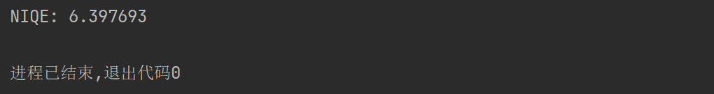
img_path = '../../../tests/data/bic/baboon.png'
crop_border=4

img = cv2.imread(img_path, cv2.IMREAD_UNCHANGED)  # [480, 500, 3]
niqe = calculate_niqe(img, crop_border=crop_border, input_order='HWC', convert_to='y')
print(f'NIQE: {niqe:.6f}')