


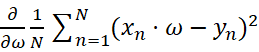
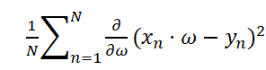
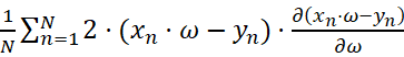
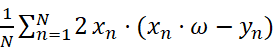
优化问题:即求loss最小值。
Gradient:![]()
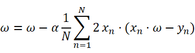
Update:![]() 其中,α称为学习率。(采用贪心策略)
其中,α称为学习率。(采用贪心策略)
在神经网络中,局部最优点比较小,但是会存在很多的鞍点,即g=0,此时就很难再进行迭代。因此,鞍点是深度学习当中最需要解决的难点。
其中,由于:
Gradient: =
= 
= 
= 
= 
∴Update:
平均梯度下降:
import numpy  as np
import matplotlib.pyplot as plt


x_data = [1.0,2.0,3.0]
y_data = [2.0,4.0,6.0]

w = 1.0   #初始权重预测

def forward(x):
        return x * w

def cost(xs,ys):
    cost = 0
    for x,y in zip(xs,ys):
        y_pred = forward(x)
        cost += (y_pred - y) **2
    return cost/len(xs)


def gradient(xs,ys):
    grad = 0
    for x,y in zip(xs,ys):
        grad += 2 * x * (x * w - y)
    return grad / len(xs)


print('Predict (before training)',4,forward(4))

epoch_list = []
cost_list = []


for epoch in range(100):
    cost_val = cost(x_data,y_data)
    grad_val = gradient(x_data,y_data)
    w -= 0.01*grad_val       #这里的学习率设置成 0.01.
    print('Epoch:',epoch,'w=',w,'loss=',cost_val)
    epoch_list.append(epoch)
    cost_list.append(cost_val)

print('Predict (after training)',4,forward(4))


plt.plot(epoch_list,cost_list)
plt.ylabel('Loss')
plt.xlabel('epoch')
plt.show()
随机梯度下降算法的Update为:![]() 其中,α称为学习率。(采用贪心策略)
其中,α称为学习率。(采用贪心策略)
对应的Loss Function: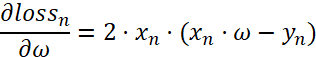
#随机梯度下降算法
import numpy  as np
import matplotlib.pyplot as plt


x_data = [1.0,2.0,3.0]
y_data = [2.0,4.0,6.0]

w = 1.0   #初始权重预测

def forward(x):
        return x * w

def loss(xs,ys):    #这里变换成loss,可去掉原先的cost = 0
      y_pred = forward(x)
      return  (y_pred - ys) **2


def gradient(xs,ys):
    return 2 * xs *(xs * w - ys)


print('Predict (before training)',4,forward(4))

epoch_list = []
loss_list = []


for epoch in range(100):
    for x,y in zip(x_data,y_data):
        grad_val = gradient(x,y)
        w -= 0.01*grad_val
        print('\tgrad:',x,y,grad_val)
        l = loss(x,y)

    print('progress:',epoch,'w=',w,'loss=',l)
    epoch_list.append(epoch)
    loss_list.append(l)

print('Predict (after training)',4,forward(4))


plt.plot(epoch_list,loss_list)
plt.ylabel('Loss')
plt.xlabel('epoch')
plt.show()
之后会采用Batch_size来平衡时间和性能之间的关系。


 1077
1077


 被折叠的 条评论
为什么被折叠?
被折叠的 条评论
为什么被折叠?
 到【灌水乐园】发言


