预测销售XGBoost

写在开头

草稿箱里面很多文章都是初稿，是之前在学习相关内容的时候写的，本身就是做备忘录了，准备这段时间把草稿箱里面的文章发出去。

项目介绍

数据集介绍

提供每日历史销售数据。 任务是为测试集预测每个商店销售的产品总量。 请注意，商店和产品列表每个月都会略有变化。 创建一个可以处理此类情况的稳健模型是挑战的一部分。

文件描述

• sales_train.csv - 训练集。 2013 年 1 月至 2015 年 10 月的每日历史数据。
• test.csv - 测试集。 您需要预测这些商店和产品在 2015 年 11 月的销售额。
• sample_submission.csv - 格式正确的样本提交文件。
• items.csv - 有关商品/产品的补充信息。
• item_categories.csv - 有关项目类别的补充信息。
• shops.csv- 有关商店的补充信息。

字段介绍

• ID - 表示测试集中的 (Shop, Item) 元组的 Id
• shop_id - 一家商店的独特标识符
• item_id - 产品的唯一标识符
• item_category_id - 项目类别的唯一标识符
• item_cnt_day -销售的产品数量。 您正在预测此措施的每月金额
• item_price - 商品的价格
• date - 日期的格式为 dd/mm/yyyy
• date_block_num - 一个连续的月份数，为方便起见。 2013 年 1 月为 0，2013 年 2 月为 1，…，2015 年 10 月为 33
• item_name - 物品的名字
• shop_name - 商店的名字
• item_category_name - 商品的种类

评估指标

提交的内容通过均方根误差 (RMSE) 进行评估。 真正的目标值被裁剪到 [0,20] 范围内。

FE

处理数据

import numpy as np 
import pandas as pd 
import matplotlib.pyplot as plt
import seaborn as sns

from sklearn.model_selection import train_test_split
import xgboost as xgb
import warnings
warnings.filterwarnings("ignore", category=UserWarning)
%matplotlib inline

• 读取数据

df_sales = pd.read_csv('sales_train.csv')
df_items = pd.read_csv('items.csv')
df_shops = pd.read_csv('shops.csv')
df_test = pd.read_csv('test.csv')
df_sub = pd.read_csv('sample_submission.csv')

• 去重

df_sales.drop_duplicates(keep='first', inplace=True, ignore_index=True)

df_sales.shape

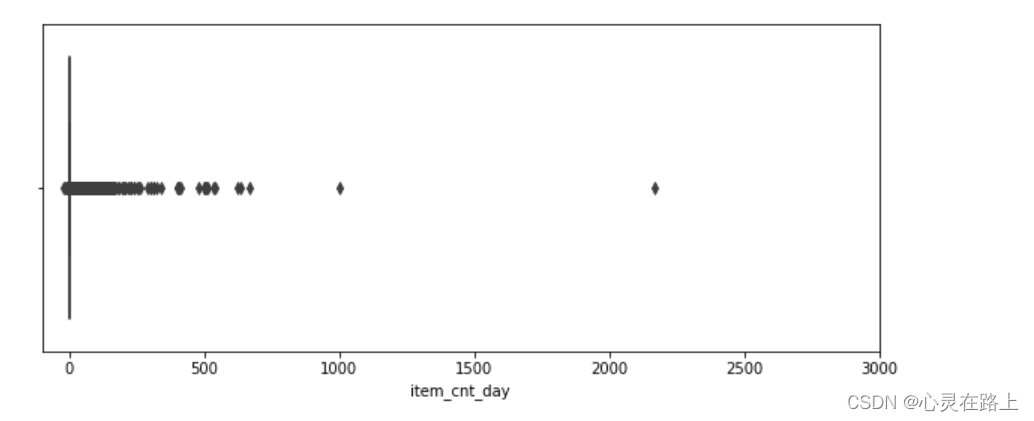
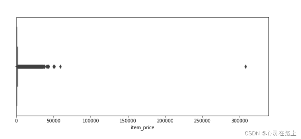
• 看下有没有异常值

plt.figure(figsize=(10,4))
plt.xlim(-100, 3000)
sns.boxplot(x=df_sales.item_cnt_day)

plt.figure(figsize=(10,4))
plt.xlim(df_sales.item_price.min(), df_sales.item_price.max()*1.1)
sns.boxplot(x=df_sales.item_price)

• 去除异常值

df_sales[df_sales['item_price'] <0]

df_sales.drop(df_sales[df_sales['item_cnt_day'] <0].index , inplace=True)
df_sales.drop(df_sales[df_sales['item_price'] <0].index , inplace=True)

df_sales.shape

• 这里使用四分差处理异常值

Q1 = np.percentile(df_sales['item_price'], 25.0)
Q3 = np.percentile(df_sales['item_price'], 75.0)

IQR = Q3 - Q1

df_sub1 = df_sales[df_sales['item_price'] > Q3 + 1.5*IQR]
df_sub2 = df_sales[df_sales['item_price'] < Q1 - 1.5*IQR]

df_sales.drop(df_sub1.index, inplace=True)

df_sales.shape

• 这里是想使用平均价格来做后续计算的依据。
  首先查看下每个月份销售的平均价格

dict(round(df_sales.groupby('date_block_num')['item_price'].mean(),4))

• 看下每个月销售的平均价格

price = round(np.array(df_sales.groupby('date_block_num')['item_price'].mean()).mean(),2)
print(price)

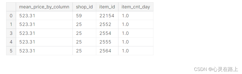
处理特征

• 这里开始处理

replace_dict = dict(round(df_sales.groupby('date_block_num')['item_price'].mean(),2))
df_sales['date_block_num'] = df_sales['date_block_num'].replace(replace_dict)

df_train = df_sales.copy()
df_train.drop(['date','item_price'], axis=1, inplace=True)
df_train.rename(columns = {'date_block_num':'mean_price_by_column'}, inplace=True)
df_train.head()

mean_price = np.array(df_sales.groupby('date_block_num')['item_price'].mean()).mean()

com_df = pd.concat([df_train,df_test])

com_df['mean_price_by_column'] = com_df['mean_price_by_column'].fillna(value=price)
com_df['item_cnt_day'] = com_df['item_cnt_day'].fillna(value=0)

test_df = com_df[com_df['item_cnt_day'] == 0]
train_df = com_df[com_df['item_cnt_day'] != 0]

traindf = train_df.copy()
traindf.drop('ID', inplace=True, axis=1)

testdf = test_df.copy()

testdf.drop('ID', inplace=True, axis=1)
testdf.drop('item_cnt_day', inplace=True, axis=1)

traindf = train_df.copy()
traindf.drop('ID', inplace=True, axis=1)
traindf['item_id'] = (traindf['item_id'] - traindf['item_id'].mean())/traindf['item_id'].std()

建模和评估

这里只写了xgboost的代码，lightgbm和catboost 的代码可以在下面的代码基础上直接修改就好了。

XGboost

代码

X_train, X_valid, y_train, y_valid = train_test_split(X, y,train_size=0.8, random_state= 42)

dtrain = xgb.DMatrix(data=X_train,label=y_train)
dtest = xgb.DMatrix(data=X_valid,label=y_valid)



model = xgb.XGBRegressor(
    max_depth=8,
    n_estimators=100,
    min_child_weight=30, 
    colsample_bytree=0.8, 
    subsample=0.8, 
    eta=0.1,    
    seed=42,
    eval_metric="rmse",
    validate_parameters = False,
    early_stopping_rounds = 10,
    verbosity=0,
)

# res = xgb.cv(model.get_params(), dtrain, num_boost_round=10, nfold=5,
#              callbacks=[xgb.callback.EvaluationMonitor(show_stdv=False),
#                         xgb.callback.EarlyStopping(3)])
fit_model = model.fit(
    X_train, 
    y_train, 
    eval_set=[(X_train, y_train), (X_valid, y_valid)], 
    verbose=True,)

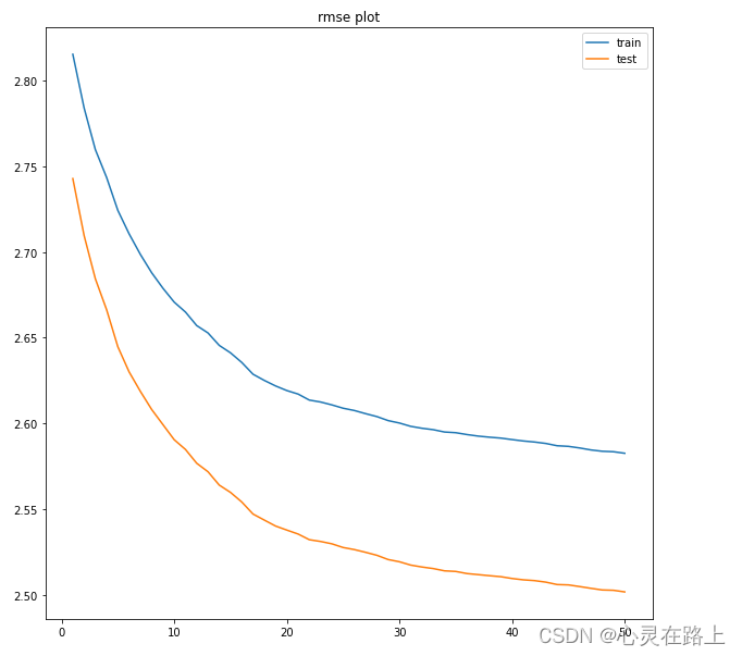
可视化

# cv的可视化
plt.figure(figsize=(10,10))
plt.plot(np.arange(1,res.shape[0]+1,1), res["train-rmse-mean"])
plt.plot(np.arange(1,res.shape[0]+1,1), res["test-rmse-mean"])
plt.title("rmse plot")
plt.legend(['train','test']) #打出图例
plt.show()

hyperopt +XGBoost

代码

import hyperopt
from hyperopt import fmin, tpe, hp, partial
from sklearn.model_selection import train_test_split, cross_val_score
from sklearn.metrics import mean_squared_error, zero_one_loss
import warnings
warnings.filterwarnings(action='ignore', category=UserWarning)



train_rmse_list = []
test_rmse_list = []

def hyperopt_objective(params):
    global train_rmse_list
    global test_rmse_list
    
    model = xgb.XGBRegressor(
        max_depth=int(params['max_depth'])+1,
        learning_rate=params['learning_rate'],
        n_estimators=params['n_estimators'],
        silent=1,
        objective='reg:squarederror',
        eval_metric='rmse',
        seed=42,
        nthread=-1,
        enable_categorical = False,
        verbosity=0,
    )
     
    res = xgb.cv(model.get_params(), dtrain, num_boost_round=10, nfold=5,verbose_eval = True
             )
    train_rmse_list += list(res["train-rmse-mean"])
    test_rmse_list += list(res["test-rmse-mean"])
    
    return np.min(res['test-rmse-mean']) # as hyperopt minimises

from numpy.random import RandomState

params_space = {
    'max_depth': hp.randint('max_depth', 6),
    'learning_rate': hp.uniform('learning_rate', 1e-3, 5e-1),
    "n_estimators": hp.randint("n_estimators", 300),
}

trials = hyperopt.Trials()

best = fmin(
    hyperopt_objective,
    space=params_space,
    algo=hyperopt.tpe.suggest,
    max_evals=10,
    trials=trials,
)

print("\n展示hyperopt获取的最佳结果，但是要注意的是我们对hyperopt最初的取值范围做过一次转换")
print(best)

可视化

plt.figure(figsize=(10,10))
plt.plot(np.arange(1,len(train_rmse_list)+1,1), train_rmse_list)
plt.plot(np.arange(1,len(test_rmse_list)+1,1), test_rmse_list)
plt.title("rmse plot")
plt.legend(['train','test']) #打出图例
plt.show()

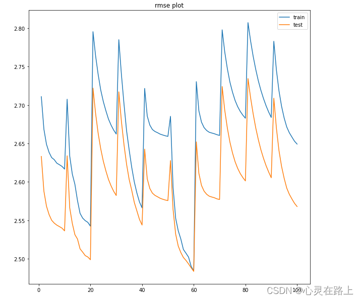
回顾：

• 本次处理没有考虑商店新品，也就是商品销售为0的情况；
• 调参的范围还是有待商榷，RMSE值比较高，还有优化的空间。