Optimizing Generated HDL Code学习

目标：

1. 满足时序要求通过流水线方式。

2.选择具体的硬件实现方式，比如FPGA的具体型号。

3.比特级循环交叉验证正确性。

核心：还是在于关键路径的缩短——尽量处理较少的组合逻辑。

Example one:

Square Root Implementation

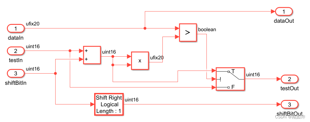
平方根算法：首先将带开方的数进行二进制转换，位数拼接多一点，16位左右。然后再找一个数移位从大到小与输出值相加，相加后平方。再与原来的数进行比较大小，小了，就取相加后的数；大了，就取相加之前的数。循环迭代，最后输出开方值。

评价：乘法器多，循环次数多，精度有待考虑。

Example Two

HDL Workflow Advisor

1.首先输入代码hdlsetuptoolpath('ToolName', 'Xilinx Vivado', ...

'ToolPath', 'D:\Vivado\Vivado\2018.3\bin');%%作用是将电脑的vivado软件路径添加到Matlab。

2.然后进入Simulink软件，打开HDL Workflow Advisor选项，确认识别成功。

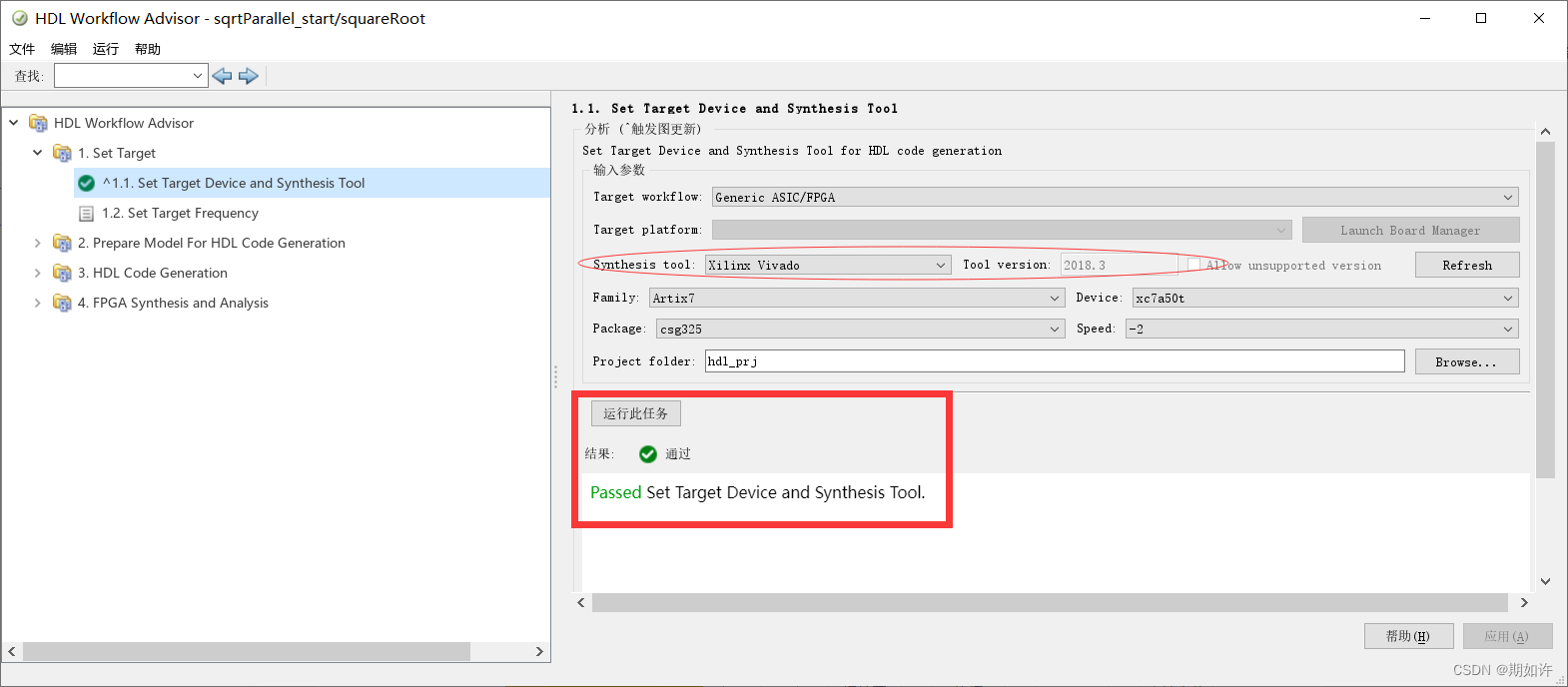
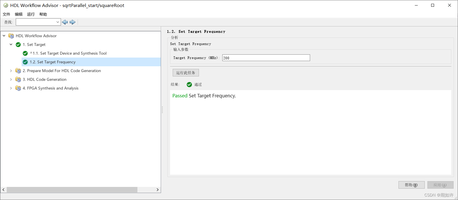
3.Setting Target Frequency，产生时钟约束文件.xdc，每个周期组合逻辑时间 ≤ 5ns。

数据的采样率和时钟频率后文会详细分析，there is often a difference ! 

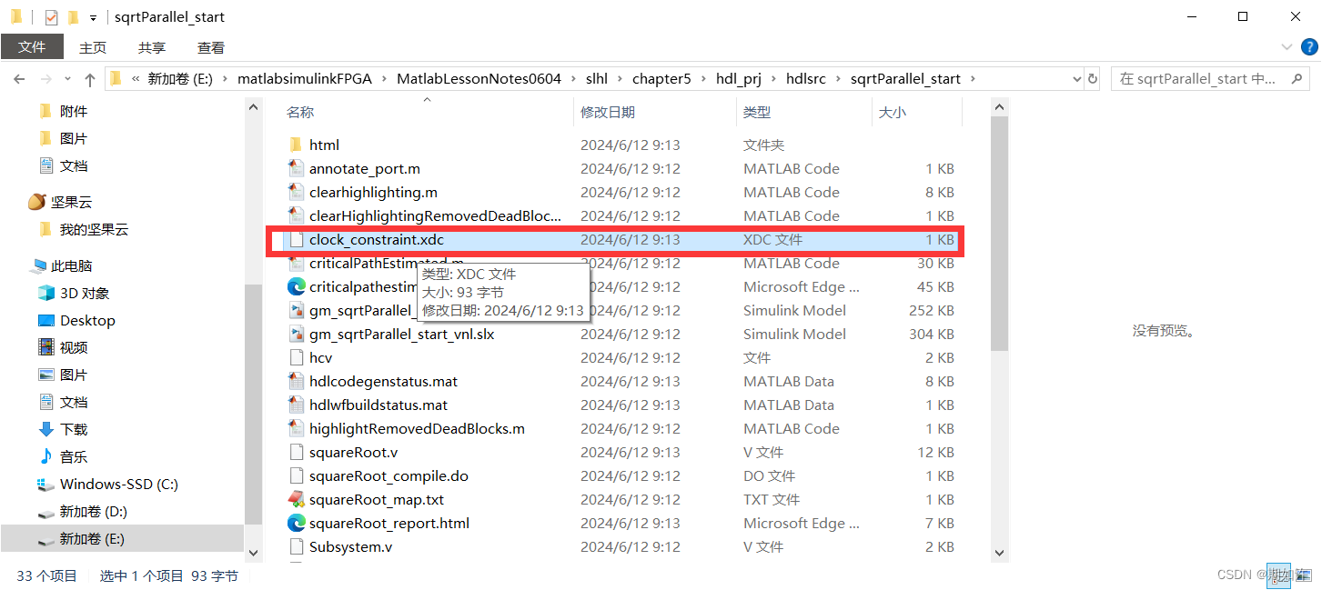
4.生成HDL Code，这里我们主要是用verilog语言，文件后缀.v文件。

5.继续关注时序分析，打开critical path estimation报告，点击Hignlight Critical Path。

我们可以看到最长的关键路径的可视化，在模型当中。

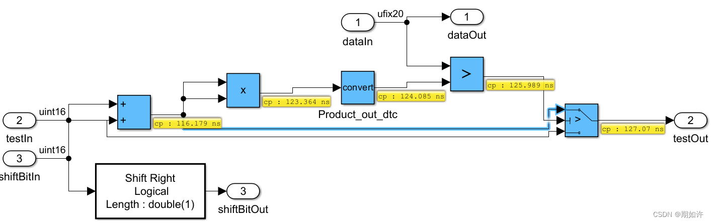
深蓝色标志着关键路径，但不代表结束，因为还有更高层，还需要从testout出去看。

显然，是不满足时序要求的，哈哈。

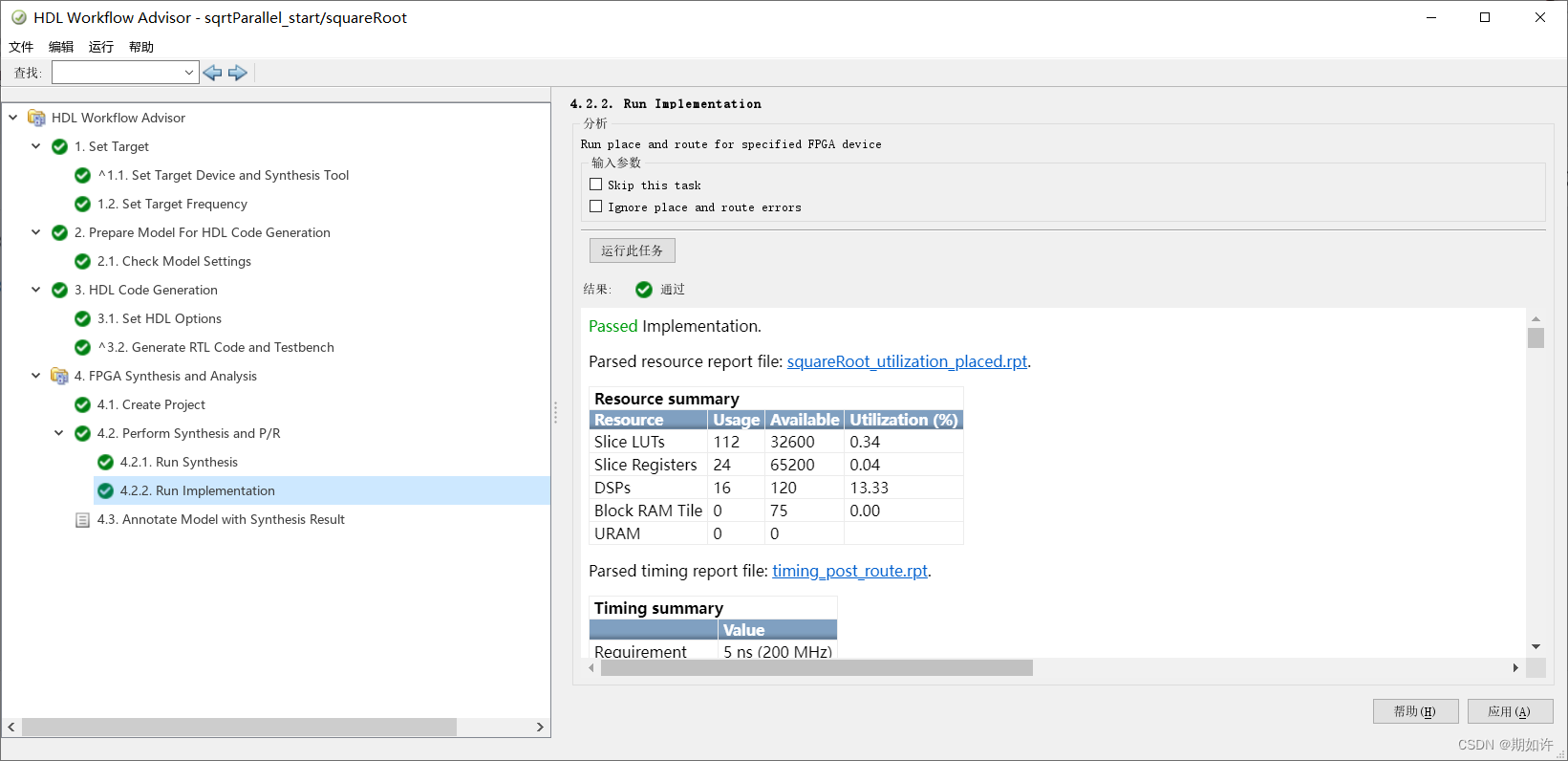
6.vivado嵌入simulink中的综合与实现。synthesis and implementation。

默认情况下，skip implementation操作，但是最准确的时序分析是在"实现"之后完成。

可以手动点击运行，先综合再实现。“实现”的时间会特别漫长.......

Exmaple Three

Pipelining

1.解决时序问题的方法就是加寄存器，这里一般说加流水线。

2.可以手动加一个Delay 或者 自适应加延时（根据设置的设备和频率）。

3.Block properties.

4.Distributed Pipelining.

Example Four

自适应加延时方法演示

使用前：已经有一个小小的模块，最好定点化完成了，但是时延没通过，流水线也没加。

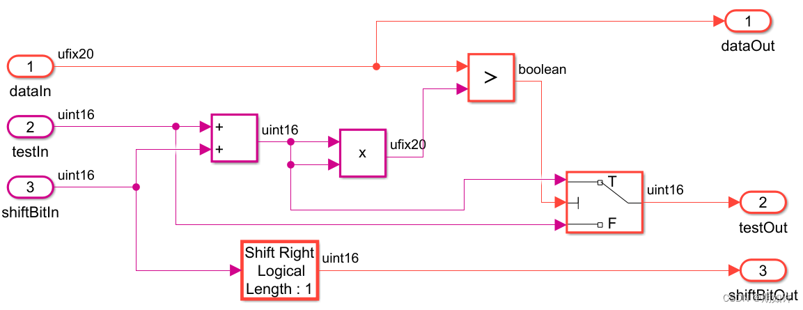
现在，把设置里面>最优化>流水线>勾选自适应流水线，打开Workflow Advisor。

一直运行，直到全绿，打开代码生成报告。

最下方上面一点点的是对比模型，点击最下方的生成模型（已经最新优化结果），非常的哇塞！

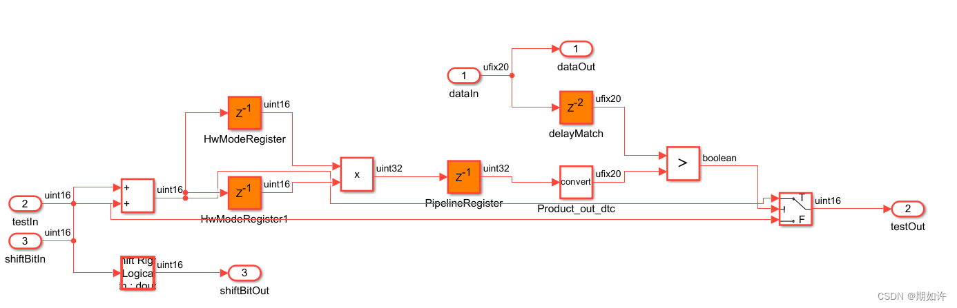
最直观的一点就是乘法器前后都加了Delay，非常智能。

遇到HwModelRegister模块是z-d现象，也是正常的，刷新一下，因为没有hdlsetup。

我们再看一下关键路径：

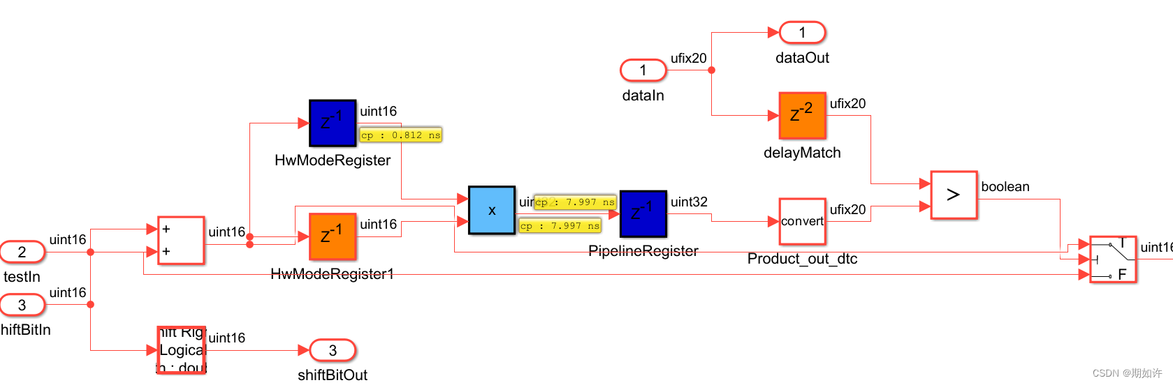
非常的清晰！

乘法器的时延非常大，但是映射到专用DSP硬件上其实时延会小很多。

实际上的vivado软件里面synthesis和Implementation之后延时会小很多。

Synthesis                 Slack         0.508ns

Implementation        Slack         0.233ns

务必找到Timing Summary Report文件

保存位置在vivado_prj工程文件目录下的.rpt文件名，但是在Matlab里面记得要拖拽打开。

总的资源利用表格和时序分析报告都在下面这个根目录下：

hdl_prj\vivado_prj\slprj

到此为止，完成时序优化，满足时序需求，关键路径实现时间在5ns周期内。

小结

手动delay也行

自适应delay也行

最后满足时序要求就可~~~