论文阅读 (35)：Spatial Transformer Networks

引入

  题目：Spatial transformer networks
  演示：https://goo.gl/qdEhUu
  代码：
  摘要：卷积神经网络定义了一类有力模型，但依然受到输入数据空间不变 (spatially invariant)的限制。本文引入一个新的可学习模块，即空间转换器 (spatial transformer)，其明确允许在网络内对数据进行空间操作。该可微分模块可以应用到现有的卷积架构中，使得网络能够主动空间变换特征图，而无需额外的监督训练，或优化更改。本文验证了空间转换器的使用，可以使得模型习得平移、缩放、旋转和更通用变换的不变性 (invariance)，且相较于其他变换器有优势。
  Bib：

@article{Jaderberg:2015:20172025,
author		=	{Max Jaderberg and Karen Simonyan and Andrew Zisserman and Koray Kavukcuoglu},
title		=	{Spatial transformer networks},
journal		=	{Advances in Neural Information Processing Systems},
volume		=	{28},
year		=	{2015},
pages		=	{2017--2025}
}

1 空间转换器 (spatial transformer)

  空间转换器是一个可微分模块，可用于单次前向传递期间，对特征图的空间变换，其中变换以特定输入为条件，并产生单个特征图输出。对于多通道输入，每个通道应用相同的变换。本节仅考虑单个变换和每个变换器的单个输出，多个变换的推广则在实验进行。
  空间转换器可分为三个部分，如图2：
  1）定位网络 (localisation network)：获取输入特征图，并通过多个隐藏层输出应该应用于特征图的空间变化参数；
  2）网格生成器 (grid generator)：使用预测的空间变换参数创建采样网格，其是一组点的集合；
  3）采样器 (sampler)：以特征图和采样网格作为输出，生成从网格点输入的采样输出图。

图2：空间转换器

1.1 定位网络 (localisation network)

  输入：特征图$U\in {\mathbb{R}}^{H\times W\times C}$，其中$H$、$W$、$C$分别对应高、宽、通道。
  输出：变换${\mathcal{T}}_{\theta }$的参数$\theta$，其可用于特征图，即$\theta =f_{\text{loc}}(U)$，其大小根据变换的类型而变化。$f_{\text{loc}}(\cdot )$是一个可以采用任何形式的定位网络，例如一个全连接网络或者卷积网络，但应该包含一个最终的回归层 (regression layer)，以生成变换参数$\theta$。

1.2 参数化采样网格 (parameterised sampling grid)

  为了对输入特征图进行变换，每个像素都使用以输入特征图为中心的采样核的计算。在这里，像素作为通用特征图的元素而不一定是图像。通常，输出像素被定义为位于像素$G_i=(x_i^t,y_i^t)$上的规则网格 G = { G i } G=\{G_i\} G={Gi​}。所有的网格构成输出特征图$V\in {\mathbb{R}}^{H^{\prime }\times W^{\prime }\times C}$。注意当前步骤的输入输出形状一致。
  为了清楚描述，暂时假设${\mathcal{T}}_{\theta }$是一个2D仿射变换$A_{\theta }$。此时的逐点变换 (pointwise transformation)为
$$\left(\begin{array}{c}{x}_i^s\\ y_i^s\end{array}\right)={\mathcal{T}}_{\theta }(G_i)=A_{\theta }\left(\begin{array}{c}{x}_i^s\\ y_i^s\\ 1\end{array}\right)=\left[\begin{array}{ccc}{\theta }_{11}& {\theta }_{12}& {\theta }_{13}\\ {\theta }_{21}& {\theta }_{22}& {\theta }_{23}\end{array}\right]\left(\begin{array}{c}{x}_i^s\\ y_i^s\\ 1\end{array}\right)\text{\hspace{1em}(1)}$$其中$(x_i^t,y_i^t)$规则网格在输出特征图上的目标坐标，$(x_i^s,y_i^s)$定义了采样点的、在输入特征图上的源坐标。我们使用高和宽来标准化坐标，使得$-1\le x_i^t,y_i^t\le 1$以及$-1\le x_i^s,y_i^s\le 1$。源/目标变换和采样相当于图像中使用的标准纹理映射和坐标。
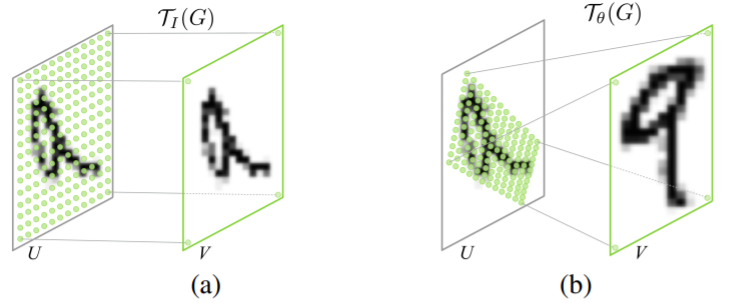
  公式1中定义的变换允许对输入特征图应用裁剪、平移、旋转、缩放和倾斜，并且只需要定位网络生成$A_{\theta }$的六个参数。进一步，其允许裁剪的原因是，如果变换是收缩 (contraction)，那么映射的规则网格将位于面积小于$s$范围的平行四边形中。图3展示了该变化与恒等变换的区别。

图3：公式1定于的变换与恒等变换的区别

 
  事实上，${\mathcal{T}}_{\theta }$可以有更多的约束，例如
$$A_{\theta }=\left[\begin{array}{ccc}s& 0& t_x\\ 0& s& t_y\end{array}\right]\text{\hspace{1em}(2)}$$其允许裁剪、平移和各向同性缩放。该变换也可以更具普适性，例如基于八个参数的屏幕投影、分段放射和thin plate spline。事实上，该变换可以有任何的参数形式，只要它在参数方面是可微的。

1.3 可微图像采样 (differentiable image sampling)

  为了对输入特征图进行空间变换，采样器必须保有点集${\mathcal{T}}_{\theta }(G)$、输入特征图$U$、采样输出特征图$V$。
  ${\mathcal{T}}_{\theta }(G)$上的每一个点$(x_i^s,y_i^s)$定义了一个应用了采样核的输入上的空间坐标，这里采样核用于获取给定像素在输入$V$上的特定值，可以记作：
$$V_i^c=\sum _n^H\sum _m^W{U}_{nm}^{c}k\left(x_i^s-m;{\Phi }_x\right)k\left(y_i^s-n;{\Phi }_y\right)\forall i\in \left[1\dots H^{\prime }{W}^{\prime }\right]\forall c\in [1\dots C]\text{\hspace{1em}(3)}$$其中${\Phi }_x$和${\Phi }_y$是定义了图像差值的采样核$k()$的参数，$U_{nm}^c$是输入$c$通道上的坐标$(n,m)$，$V_i^c$是输出$c$通道上坐标$(x_i^t,y_i^t)$的像素$i$。注意输入的每个通道进行了相同的采样，因此每个通道都进行了相同的变换，这保证了多个通道之间的空间一致性。
  理论上，在可以相对于$x_i^s$和$y_i^s$定义梯度，任意的采样核都可以被使用。例如使用整数采样核时，我们有：
$$V_i^c=\sum _n^H\sum _m^W{U}_{nm}^c\delta \left(\lfloor x_i^s+0.5\rfloor -m\right)\delta \left(\lfloor y_i^s+0.5\rfloor -n\right)\text{\hspace{1em}(4)}$$其中$\delta ()$是Kronecker增量函数。这个采样核等价于将$(x_i^s,y_i^s)$的近邻点复制给$(x_i^t,y_i^t)$。采用双线性采样核时：
$$V_i^c=\sum _n^H\sum _m^W{U}_{nm}^c\max \left(0,1-\left|x_i^s-m\right|\right)\max \left(0,1-\left|y_i^s-n\right|\right)\text{\hspace{1em}(5)}$$其关于$U$和$G$的偏导定义为：
$$\begin{array}{c}\frac{\partial V_i^c}{\partial U_{nm}^c}=\sum _n^H\sum _m^W\max \left(0,1-\left|x_i^s-m\right|\right)\max \left(0,1-\left|y_i^s-n\right|\right)\\ \frac{\partial V_i^c}{\partial x_i^s}=\sum _n^H\sum _m^W{U}_{nm}^c\max \left(0,1-\left|y_i^s-n\right|\right)\{\begin{array}{ll}0& \text{ if }\left|m-x_i^s\right|\ge 1\\ 1& \text{ if }m\ge x_i^s\\ -1& \text{ if }m<x_i^s\end{array}\end{array}\text{\hspace{1em}(7)}$$其中$\frac{\partial V_i^c}{\partial x_i^s}$是类似的。这使得反向传播是可行的。