机器学习识别系统的度量指标

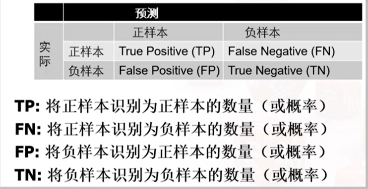
混淆矩阵

在使用支持向量机模型进行分类时：如果调整判断的阈值，如


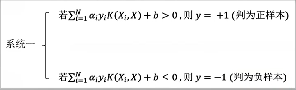
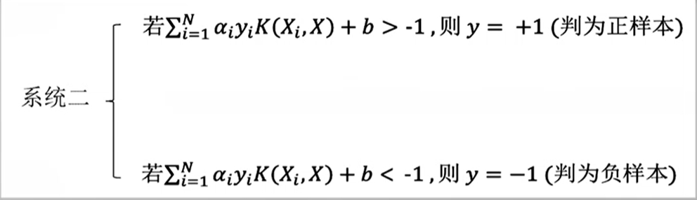
则TP，FP均增加。这是因为将判别的阈值改为-1，则会有更多的测试样本被判别为正样本，则TP，FP均增加。

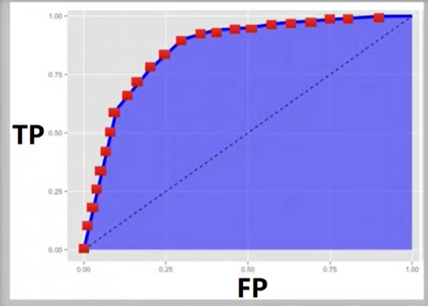
ROC曲线

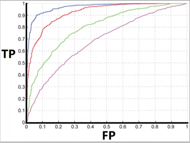
AUC

代表右下角面积，越大代表分类效果越好。

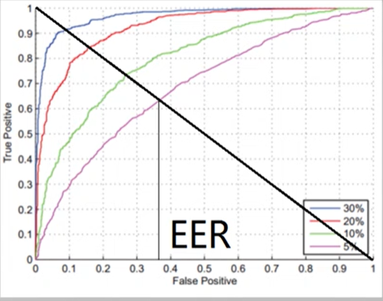
EER

等错误率。FP=FN

下面是对于兵王问题利用SVM来进行二分类的程序：
首先是对数据集进行一个分析和处理：

'''
总样本数28056，其中正样本2796，负样本25260.
随机选取5000个样本训练，其余测试。
将draw设置为+1，其他为-1
'''
s = open('krkopt.data','r',encoding='utf-8')
x_data = []
y_data = []
for i in s.readlines():
    i = i.rstrip().split(',')
    if i[0]=='??': break
    y_data.append(1 if i[-1] == "draw" else -1)
    xs =[]
    for k in i[:-1]:
        xs.append(int(k) if k.isalpha()==False else (ord(k)-ord('a')+1))
    x_data.append(xs)
s.close()

然后进行归一化

#归一化
import pandas as pd
ds = pd.DataFrame(x_data,columns={'pbx','pby','pr1x','pr1y','pr2x','pr2y'})
columnname = [i for i in ds]
for i in columnname:
    ds[i] = (ds[i]-ds.describe()[i]['mean'])/(ds.describe()[i]['std'])
ds = ds.values
print(ds.shape)
print(len(y_data)

进行随机选取，得到训练集

import numpy as np
ds_x =[]
ds_y =[]
for i in range(2500):
    ind = np.random.randint(0, 2800)
    ds_x.append(ds[ind])
    ds_y.append(y_data[ind])
for i in range(2500):
    ind = np.random.randint(2800, 25260)
    ds_x.append(ds[ind])
    ds_y.append(y_data[ind])
print(ds_x[:5])
print(ds_y[:5])

进行SVM的训练和评估

from sklearn import svm
#3.训练svm分类器
classifier=svm.SVC(C=2,kernel='rbf',gamma=10,decision_function_shape='ovr') # ovr:一对多策略
#参数详解见https://blog.csdn.net/weixin_41990278/article/details/93137009
classifier.fit(ds_x,ds_y)

#4.计算svc分类器的准确率
print("训练集：",classifier.score(ds_x,ds_y))
print("测试集：",classifier.score(ds,y_data))
训练集： 1.0
测试集： 0.9668876532648988

#查看决策函数
print('train_decision_function:',classifier.decision_function(ds_x))
print('predict_result:',classifier.predict(ds_x))

计算混淆矩阵

#计算评价指标。
pred = classifier.predict(ds)
print(pred.shape)
correct = np.equal(y_data[:2796], pred[:2796])
TP = np.mean(correct.astype(np.float))
FN = 1-TP
correct_TN = np.equal(y_data[2796:], pred[2796:])
TN = np.mean(correct_TN.astype(np.float))
FP = 1-TN
matrix = [[TP, FN], [FP, TN]]
matrix = pd.DataFrame(matrix, columns=['正样本','负样本'])
matrix.index=['实际正样本','实际负样本']
print(matrix)
'''
 正样本       负样本
实际正样本  0.879471  0.120529
实际负样本  0.023436  0.976564
'''       

改进版本

参考了一份代码，地址：https://www.yuque.com/docs/share/97eb71c5-2715-40af-b873-a61785175b98?#

#数据预处理与导包，里面有几个非常好用的函数。
import numpy as np
import pandas as pd
import matplotlib.pyplot as plt
import matplotlib

%matplotlib inline
matplotlib.rcParams.update({'font.size': 20})

from sklearn.model_selection import train_test_split
from sklearn.svm import SVC
from sklearn.preprocessing import StandardScaler
from sklearn.model_selection import GridSearchCV
from sklearn.metrics import confusion_matrix

from sklearn.metrics import roc_curve


# 读取数据
names = ['x1', 'y1', 'x2', 'y2', 'x3', 'y3', 'label']
data = pd.read_csv('krkopt.data', names=names)
data.head()

# 处理数据
letter_num_map = {
    "a": 1,
    "b": 2,
    "c": 3,
    "d": 4,
    "e": 5,
    "f": 6,
    "g": 7,
    "h": 8,
    "draw": 1,
    "zero": -1,
    "one": -1,
    "two": -1,
    "three": -1,
    "four": -1,
    "five": -1,
    "six": -1,
    "seven": -1,
    "eight": -1,
    "nine": -1,
    "ten": -1,
    "eleven": -1,
    "twelve": -1,
    "thirteen": -1,
    "fourteen": -1,
    "fifteen": -1,
    "sixteen": -1
}
for i in ["x1", "x2", "x3", "label"]:
    data[i] = data[i].map(lambda x: letter_num_map.get(x, 0))
    
# 查看数据
data.head()
data.info()
data.describe()

# 查看label分布
data.label.value_counts()
data.label.hist(figsize=(10, 5))
plt.title('Class counts')

# 将数据集分割为训练集和测试集
X = data.iloc[:, :-1]
y = data.iloc[:, -1]
# random_state 指定随机数seed
X_train, X_test, y_train, y_test = train_test_split(X, y, train_size=5000, random_state=0)

print(X_train.shape)
print(y_train.shape)

在进行SVM训练时，用到了GridSearchCV()方法。
参考资料：https://blog.csdn.net/foneone/article/details/89985045
下面这里C与gamma的范围可以根据需要调整，这里我没有改变参数，训练的时间比较长。

# 归一化
scaler = StandardScaler()
scaler.fit(X_train)
X_train_scaled = scaler.transform(X_train)
X_test_scaled = scaler.transform(X_test)

# Grid Search with Cross-Validation
# 选用高斯核函数
param_grid = {'C': list(map(lambda x: 2 ** x, range(-5, 16))),
              'gamma': list(map(lambda x: 2 ** x, range(-15, 4)))}
print(f"Parameter grid:\n {param_grid}")

# 训练 耗时操作需要等待
grid_search = GridSearchCV(SVC(), param_grid, cv=5)
grid_search.fit(X_train_scaled, y_train)

#评估 包括最佳参数得到的准确率和混淆矩阵，以及多个参数得到的ROC曲线。
# 测试准确率
print("Test set score: {:.4f}".format(grid_search.score(X_test_scaled, y_test)))
print("Best parameters: {}".format(grid_search.best_params_))

# 查看混淆矩阵

def plot_confusion_matrix(grid_search, x_test, y_test):
    fig = plt.figure(figsize=(10,10))
    ax = fig.add_subplot(1, 1, 1)
    y_pred = grid_search.predict(x_test)
    Carray = confusion_matrix(y_test, y_pred) #C中为TP FP TN FN 的值
    TP = Carray[0][0] / (Carray[0][0]+Carray[0][1])
    FN = 1-TP
    FP = Carray[1][0] /(Carray[1][0] +Carray[1][1])
    TN = 1-FP
    Cmat = [[TP, FN] ,[FP , TN]]
    Cmat = pd.DataFrame(Cmat, columns=['预测正样本','预测负样本'])
    Cmat.index=['实际正样本','实际负样本']
    print(Cmat)

plot_confusion_matrix(grid_search, X_test_scaled, y_test)

# 绘制ROC曲线
def plot_roc_curve(grid_search, x_test, y_test):
    y_score = grid_search.decision_function(x_test)
    fpr,tpr,threshold = roc_curve(y_test, y_score) ###计算真正率和假正率
    roc_auc = auc(fpr,tpr) ###计算auc的值
    lw = 2
    plt.plot(fpr, tpr, color='darkorange',
         lw=lw, label='ROC curve (area = %0.2f)' % roc_auc) ###假正率为横坐标，真正率为纵坐标做曲线
    plt.plot([0, 1], [0, 1], color='navy', lw=lw, linestyle='--')
    plt.xlim([0.0, 1.0])
    plt.ylim([0.0, 1.05])
    plt.xlabel('False Positive Rate')
    plt.ylabel('True Positive Rate')
    plt.title('Receiver operating characteristic example')
    plt.legend(loc="lower right")
    plt.show()
    print(roc_auc) #输出roc的值。
plot_roc_curve(grid_search, X_test_scaled, y_test)

AUC值为0.997313.

参考

https://blog.csdn.net/u012679707/article/details/80511968
//利用SVM对Iris.data进行分类。
https://blog.csdn.net/weixin_41990278/article/details/93137009
//参数SVM参数详解
https://blog.csdn.net/xyz1584172808/article/details/81839230//ROC
https://blog.csdn.net/foneone/article/details/89985045//GridSearchCV
https://blog.csdn.net/u011734144/article/details/80277225//confusion_matrix