Python 数据科学 Pandas 基础

Pandas 是基于 Numpy 创建的 Python 库，为 Python 提供了易于使用的 数据结构和 数据分析工具。

 

使用以下语句导入 Pandas 库：

import pandas as pd

Pandas 数据结构

Series - 序列

存储任意类型数据的一维数组

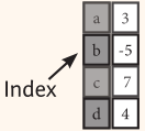
s = pd.Series([3, -5, 7, 4], index=['a', 'b', 'c', 'd'])

DataFrame - 数据框

存储不同类型数据的二维数组

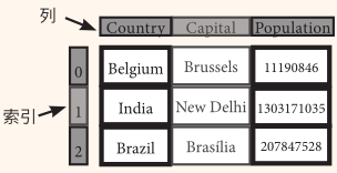
data = {'Country': ['Belgium', 'India', 'Brazil'], 
        'Capital': ['Brussels', 'New Delhi', 'Brasília'],
        'Population': [11190846, 1303171035, 207847528]}
df = pd.DataFrame(data, columns=['Country', 'Capital', 'Population'])

调用帮助

help(pd.Series.loc)

选择

取值

s['b'] # 取序列的值

#输出结果为

-5

df[1:] # 取数据框的子集

#输出结果为


    Country	Capital	Population
1	India	New Delhi	1303171035
2	Brazil	Brasília	207847528

选取、布尔索引及设置值

按位置

df.iloc[[0],[0]] # 按行与列的位置选择某值

#输出结果为


    Country
0	Belgium

按标签

df.loc[[0], ['Country']] # 按行与列的名称选择某值

#输出结果为


    Country
0	Belgium

按标签/位置

df.loc[2] # 选择某行

#输出结果为


Country          Brazil
Capital        Brasília
Population    207847528
Name: 2, dtype: object

df.loc[:,'Capital'] # 选择某列

#输出结果为


0     Brussels
1    New Delhi
2     Brasília
Name: Capital, dtype: object

df.loc[1,'Capital']

#输出结果为

'New Delhi'

 布尔索引

s[~(s > 1)] # 序列 S 中没有大于1的值

#输出结果为

b   -5
dtype: int64

s[(s < -1) | (s > 2)] # 序列 S 中小于-1或大于2的值

#输出结果为

a    3
b   -5
c    7
d    4
dtype: int64

df[df['Population']>1200000000] # 使用筛选器调整数据框

#输出结果为

	Country	Capital	Population
1	India	New Delhi	1303171035

设置值

s['a'] = 6 # 将序列 S 中索引为 a 的值设为6

删除数据

s.drop(['a', 'c']) # 按索引删除序列的值 (axis=0) 

#输出结果为

b   -5
d    4
dtype: int64

df.drop('Country', axis=1) # 按列名删除数据框的列(axis=1)

#输出结果为

    Capital	Population
0	Brussels	11190846
1	New Delhi	1303171035
2	Brasília	207847528

*只要不赋值，源数据就不会变

排序和排名

df.sort_index() # 按索引排序

#输出结果为

Country	Capital	Population
0	Belgium	Brussels	11190846
1	India	New Delhi	1303171035
2	Brazil	Brasília	207847528

df.sort_values(by='Country') # 按某列的值排序

#输出结果为

Country	Capital	Population
0	Belgium	Brussels	11190846
2	Brazil	Brasília	207847528
1	India	New Delhi	1303171035

df.rank() # 数据框排名   

#输出结果为

Country	Capital	Population
0	1.0	2.0	1.0
1	3.0	3.0	3.0
2	2.0	1.0	2.0

查询序列与数据框的信息

基本信息

df.shape # （行,列)
df.index # 获取索引
df.columns # 获取列名
df.info() # 获取数据框基本信息   
df.count() # 非Na值的数量

#输出结果为

>>>(3, 3)

>>>RangeIndex(start=0, stop=3, step=1)

>>>Index(['Country', 'Capital', 'Population'], dtype='object')

>>><class 'pandas.core.frame.DataFrame'>
RangeIndex: 3 entries, 0 to 2
Data columns (total 3 columns):
 #   Column      Non-Null Count  Dtype 
---  ------      --------------  ----- 
 0   Country     3 non-null      object
 1   Capital     3 non-null      object
 2   Population  3 non-null      int64 
dtypes: int64(1), object(2)
memory usage: 200.0+ bytes

>>>Country       3
Capital       3
Population    3
dtype: int64

 汇总

df.sum() # 合计
df.cumsum() # 累计
df.min(1)/df.max(1) # 最小值除以最大值
df.idxmin() /df.idxmax() # 索引最小值除以索引最大值
df.describe() # 基础统计数据
df.mean() # 平均值   
df.median() # 中位数

#输出结果为

>>>Country              BelgiumIndiaBrazil
Capital       BrusselsNew DelhiBrasília
Population                   1522209409
dtype: object

>>>
Country	Capital	Population
0	Belgium	Brussels	11190846
1	BelgiumIndia	BrusselsNew Delhi	1314361881
2	BelgiumIndiaBrazil	BrusselsNew DelhiBrasília	1522209409

>>>0    1.0
1    1.0
2    1.0
dtype: float64

>>>

>>>
Population
count	3.000000e+00
mean	5.074031e+08
std	6.961346e+08
min	1.119085e+07
25%	1.095192e+08
50%	2.078475e+08
75%	7.555093e+08
max	1.303171e+09

>>>Population    5.074031e+08
dtype: float64

>>>Population    207847528.0
dtype: float64

匿名函数

f = lambda x: x*2 # 应用匿名函数lambda
df.apply(f) # 应用函数
df.applymap(f) # 对每个单元格应用函数

#输出结果为

Country	Capital	Population
0	BelgiumBelgium	BrusselsBrussels	22381692
1	IndiaIndia	New DelhiNew Delhi	2606342070
2	BrazilBrazil	BrasíliaBrasília	415695056

数据对齐

内部数据对齐

如有不一致的索引，则使用NA值：

s3 = pd.Series([7, -2, 3], index=['a', 'c', 'd'])
s + s3

#输出结果为

a    13.0
b     NaN
c     5.0
d     7.0
dtype: float64

使用 Fill 方法运算

还可以使用 Fill 方法进行内部对齐运算：

s.add(s3, fill_value=0)
s.sub(s3, fill_value=2)
s.div(s3, fill_value=4)
s.mul(s3, fill_value=3)

#输出结果为

>>>a    13.0
b    -5.0
c     5.0
d     7.0
dtype: float64

>>>a   -1.0
b   -7.0
c    9.0
d    1.0
dtype: float64

>>>a    0.857143
b   -1.250000
c   -3.500000
d    1.333333
dtype: float64

>>>a    42.0
b   -15.0
c   -14.0
d    12.0
dtype: float64

 输入/输出

读取/写入CSV

df = pd.read_csv('file.csv', header=None, nrows=5)
df.to_csv('myDataFrame.csv')

读取/写入Excel

pd.read_excel('file.xlsx')
pd.to_excel('dir/myDataFrame.xlsx', sheet_name='Sheet1')

#读取内含多个表的Excel
xlsx = pd.ExcelFile('file.xls')
df = pd.read_excel(xlsx, 'Sheet1')

读取和写入 SQL 查询及数据库表

from sqlalchemy import create_engine
engine = create_engine('sqlite:///:memory:')
pd.read_sql("SELECT * FROM my_table;", engine)
pd.read_sql_table('my_table', engine)
pd.read_sql_query("SELECT * FROM my_table;", engine)
# read_sql()是 read_sql_table() 与 read_sql_query()的便捷打包器

pd.to_sql('myDf', engine)

数据重塑

透视

data2 = {'Date': ['2016-03-01', '2016-03-02', '2016-03-01', '2016-03-03', '2016-03-02', '2016-03-03',], 
        'Type': ['a', 'b', 'c', 'a', 'a', 'c'],
        'Value': [11.432, 13.031, 20.784, 99.906, 1.303, 20.784]}
df2 = pd.DataFrame(data2, columns=['Date', 'Type', 'Value'])
df2

#输出结果为

	Date	Type	Value
0	2016-03-01	a	11.432
1	2016-03-02	b	13.031
2	2016-03-01	c	20.784
3	2016-03-03	a	99.906
4	2016-03-02	a	1.303
5	2016-03-03	c	20.784

df3= df2.pivot(index='Date',
        columns='Type',  
        values='Value') # 将行变为列
df3

#输出结果为

Type	a	b	c
Date			
2016-03-01	11.432	NaN	20.784
2016-03-02	1.303	13.031	NaN
2016-03-03	99.906	NaN	20.784

透视表

df4 = pd.pivot_table(df2,
                    values='Value',  
                    index='Date',
                    columns='Type') # 将行变为列
df4

#输出结果为

Type	a	b	c
Date			
2016-03-01	11.432	NaN	20.784
2016-03-02	1.303	13.031	NaN
2016-03-03	99.906	NaN	20.784

堆栈 / 反堆栈

df5 = pd.DataFrame([[0, 1], [2, 3]],
                    index=['cat', 'dog'],
                    columns=['weight', 'height'])
df5

#输出结果为

weight	height
cat	0	1
dog	2	3

stacked = df5.stack() # 透视列标签
stacked

#输出结果为

cat  weight    0
     height    1
dog  weight    2
     height    3
dtype: int64

stacked.unstack() # 透视索引标签

#输出结果为

	weight	height
cat	0	1
dog	2	3

融合

pd.melt(df2,
        id_vars=["Date"], 
        value_vars=["Type", "Value"],
        value_name="Observations") # 将列转为行

#输出结果为

	Date	variable	Observations
0	2016-03-01	Type	a
1	2016-03-02	Type	b
2	2016-03-01	Type	c
3	2016-03-03	Type	a
4	2016-03-02	Type	a
5	2016-03-03	Type	c
6	2016-03-01	Value	11.432
7	2016-03-02	Value	13.031
8	2016-03-01	Value	20.784
9	2016-03-03	Value	99.906
10	2016-03-02	Value	1.303
11	2016-03-03	Value	20.784

迭代

df.iteritems() # （列索引，序列）键值对
df.iterrows() # （行索引，序列）键值对

高级索引

# 基础选择
df3.loc[:,(df3>1).any()] # 选择任一值大于1的列
df3.loc[:,(df3>1).all()] # 选择所有值大于1的列
df3.loc[:,df3.isnull().any()] # 选择含 NaN值的列
df3.loc[:,df3.notnull().all()] # 选择不含NaN值的列
# 通过isin选择
df[(df.Country.isin(df2.Type))] # 选择为某一类型的数值 
df3.filter(items=["a","b"])  # 选择特定值                 
# df.select(lambda x: not x%5) # 选择指定元素
# 通过Where选择
s.where(s > 0) # 选择子集
# 通过Query选择
df3.query('a > c') # 查询DataFrame

设置/取消索引

df.set_index('Country') # 设置索引
df4 = df.reset_index() # 取消索引
df = df.rename(index=str,
                    columns={"Country":"cntry",
                    "Capital":"cptl", 
                     "Population":"ppltn"}) # 重命名DataFrame列名

重置索引

s2 = s.reindex(['a','c','d','e','b'])

前向填充

df.reindex(range(4), method='ffill')

#输出结果为

	Country	Capital	Population
0	Belgium	Brussels	11190846
1	India	New Delhi	1303171035
2	Brazil	Brasília	207847528
3	Brazil	Brasília	207847528

后向填充

s3 = s.reindex(range(5), method='bfill')
s3

#输出结果为

0    3 
  1    3
  2    3
  3    3
  4    3

多重索引

import numpy as np

arrays = [np.array([1,2,3]), np.array([5,4,3])]
df5 = pd.DataFrame(np.random.rand(3, 2), index=arrays)
tuples = list(zip(*arrays))
index = pd.MultiIndex.from_tuples(tuples, 
                                      names=['first', 'second'])
df6 = pd.DataFrame(np.random.rand(3, 2), index=index)
df2.set_index(["Date", "Type"]) 

重复数据

s3.unique() # 返回唯一值
df2.duplicated('Type') # 查找重复值
df2.drop_duplicates('Type', keep='last') # 去除重复值
df.index.duplicated() # 查找重复索引

数据分组

聚合

df2.groupby(by=['Date','Type']).mean()
df4.groupby(level=0).sum()
df4.groupby(level=0).agg({'a':lambda x:sum(x)/len(x), 'b': np.sum})

转换

customSum = lambda x: (x+x%2)
df4.groupby(level=0).transform(customSum)

缺失值

df.dropna() # 去除缺失值NaN
df3.fillna(df3.mean()) # 用预设值填充缺失值NaN
df2.replace("a", "f") # 用一个值替换另一个值

合并数据

data11 = {'X1': ['a', 'b', 'c'], 
        'X2': [11.432, 1.303, 99.906]}
data1 = pd.DataFrame(data11, columns=['X1', 'X2'])

data12 = {'X1': ['a', 'b', 'd'], 
        'X3': [20.784, np.nan, 20.784]}
data2 = pd.DataFrame(data12, columns=['X1', 'X3'])

合并-Merge

pd.merge(data1, 
        data2, 
        how='left', 
        on='X1')

#输出结果为

X1	X2	X3
0	a	11.432	20.784
1	b	1.303	NaN
2	c	99.906	NaN

pd.merge(data1, 
        data2, 
        how='right', 
        on='X1')

#输出结果为

	X1	X2	X3
0	a	11.432	20.784
1	b	1.303	NaN
2	d	NaN	20.784

pd.merge(data1, 
        data2,
        how='inner',
        on='X1')

#输出结果为

X1	X2	X3
0	a	11.432	20.784
1	b	1.303	NaN

pd.merge(data1, 
        data2, 
        how='outer',
        on='X1')

#输出结果为

X1	X2	X3
0	a	11.432	20.784
1	b	1.303	NaN
2	c	99.906	NaN
3	d	NaN	20.784

连接-Join

data1.join(data2, how='right')

拼接-Concatenate

#纵向
s.append(s2) 
#横向/纵向
pd.concat([s,s2],axis=1, keys=['One','Two']) 
pd.concat([data1, data2], axis=1, join='inner')

日期

from datetime import datetime
df2['Date']= pd.to_datetime(df2['Date'])
df2['Date']= pd.date_range('2000-1-1', periods=6, freq='M')
dates = [datetime(2012,5,1), datetime(2012,5,2)]
index = pd.DatetimeIndex(dates)
end = '2012-2-5'
index = pd.date_range(datetime(2012, 2, 1), end, freq='BM')

可视化

import matplotlib.pyplot as plt
s.plot()
plt.show()

df2.plot()
plt.show()