


文章目录
一、入门知识代码
# R、RStudio安装
# https://mirrors.ustc.edu.cn/CRAN/
# https://rstudio.com/products/rstudio/download/
# 网站说明task,packages list,package page
# 界面布局、显示、中文编码问题说明

######################################################

# 包
# 包的安装
install.packages("car")
# 建议在线安装,不建议本地安装
# 包的加载
library(car)
# 单独加载包内的某个函数
# car::vif()
# 更新包
update.packages() # 更新所有包,逐个提示
# 更新指定包,以包名称作为参数即可
# 移除包
remove.packages("car")

######################################################

# 获取帮助
# 某个函数的帮助
?help
help("library")
# 某个关键词的帮助
??help
help.search("library")
# 某个package的帮助
help(package = "ggplot2")

# 获取当前工作目录
getwd()
# 设置工作目录
setwd()
# 获取文件路径
file.choose()
# read.csv(file.choose())
# 转义字符 \
# rstudio的项目(工程)创建

# 保存R文件.RData
# 直接鼠标点击
save()
save.image()
# 加载R文件
load(file.choose())

# 加载某个包内置的数据集
data()

# 列示当前环境中的对象
ls()
# 移除某个对象
rm()
# 移除所有对象
rm(list = ls())
二、数据基本知识代码
# R常用数据类型
# 数值型
123
2.34

# 字符型
"Hello, World."
'123'

# 逻辑型
TRUE
T
FALSE
F

# 判断
is.numeric(123)
is.numeric(FALSE)
is.character('123')
is.character(FALSE)
is.logical('123')
is.logical(FALSE)

# 转换
as.numeric('123')
as.numeric('转换')
as.numeric(T)
as.numeric(F)
as.character(123)
as.logical("Hello, World.")
as.logical(2)
as.logical(1)
as.logical(-2)
as.logical(2.1)
as.logical(0)


# 特殊值
NA
is.na(NA)

NULL
is.null(NULL)

NaN
is.nan(NaN)

Inf
-Inf
is.infinite(-Inf)

# 示例
2/0
-2/0
0/0

######################################################
######################################################

# R常用数据结构

# 赋值
# 对象名 <- 对象值
# =
# 快捷键 alt + -

# 向量

# 常量
pi
letters
LETTERS
month.name
month.abb

v1 <- 1:5
v2 <- c(3,2,7,4,6)
v3 <- rep(v2, times = 2)
v4 <- rep(v2, each = 2)
v5 <- rep(v2, times = 2, each = 2)
v6 <- seq(from = 2, to = 9, by = 3)
v7 <- seq(from = 2, to = 9, length.out = 3)
v8 <- seq(from = 2, by = 3, length.out = 4)

v9 <- c('aic', 'bic', 'cp')
rep(v9, each = 3)

c(T,T, F,T)

# 强制转换为同一种类型的数据
c(T, "aic")

# 向量元素名称
names(v2)
names(v2) <- v9
v2

# 向量长度
length(v9)

# 向量索引
v8[3]
v8[c(1, 3, 5)]
v8[-c(1, 4)]
v2[c('aic', 'cp')]
v1[v1%%2==1]

######################################################

# 矩阵
m1 <- matrix(
  1:6,
  nrow = 2,
  # ncol = 3,
  byrow = F,
  dimnames = list(c('r1', 'r2'),
                  c('c1', 'c2', 'c3'))
)
m1

# matrix(NA, ncol = 3, nrow = 3)

m2 <- matrix(
  c(1:6,letters[1:6]),
  nrow = 3,
  byrow = F,
  dimnames = list(c('r1', 'r2', 'r3'),
                  c('c1', 'c2', 'c3', 'c4'))
)
m2

# 行列名称
colnames(m1)
rownames(m1)
dimnames(m2)

# 维度信息
dim(m1)
ncol(m1)
nrow(m1)

# 矩阵索引
m2[1,2] # 返回向量
m2[1,] # 返回向量
m2[,2] # 返回向量
m2[1:2,2:3] # 返回矩阵
m2[c(1,3), c(2,4)]

m1['r1',] # 返回向量
m1[,'c1'] # 返回向量
m1[c('r1','r2'), c('c2','c3')] # 返回矩阵

# 转换成向量
as.vector()

# 数组
# array()
######################################################

# 列表
v1 <- 1:5
m1 <- matrix(
  1:6,
  nrow = 2,
  # ncol = 3,
  byrow = F,
  dimnames = list(c('r1', 'r2'),
                  c('c1', 'c2', 'c3'))
)
l1 <- list(com1 = v1,
           com2 = m1)
l1

# 长度信息
length(l1)

# 名称
names(l1)

# 列表索引
l1$com1 # 返回向量
l1[['com2']] # 返回矩阵
l1[[2]] # 返回矩阵

l1['com1'] # 返回列表
l1[2] # 返回列表

# 新建成分
l1$com3 <- 3:6
l1

# 释放列表
unlist()

######################################################

# 数据框(特殊的列表)
df1 <- data.frame(
  c1 = 2:5,
  c2 = LETTERS[2:5]
)
df1

# 维度信息
dim(df1)
ncol(df1)
nrow(df1)

# 行列名称
names(df1)
colnames(df1)
rownames(df1)

# 数据框索引
df1[1:2, 2] # 返回向量
df1[, 2] # 返回向量
df1[1, ] # 返回数据框

df1[, "c1"] # 返回向量
df1['1',] # 返回数据框

df1[[2]] # 返回向量
df1$c1 # 返回向量

df1[2] # 返回数据框
df1['c1'] # 返回数据框

# 新建列
df1$c3 <- 1:4
df1

# 生成用于网格搜索的数据框
expand.grid(mtry = 2:5,
            ntree = c(200, 500))
三、基本运算和常用函数代码
############################################ 基本运算

1 + 2                          # 加
3 - 2                          # 减
3 * 4                          # 乘
8 / 5                          # 除

c(1:4) / c(2:5)
c(1:6) / c(2:5) # 循环扩展

4 ^ 3                          # 幂运算 底数^指数
exp(1) # 自然常数为底的幂运算
log(x = 25, base = 5) # 5为底25的对数
sqrt(4) # 开平方
abs(-5.6) # 绝对值
sign(-5.6) # 符号函数
round(3.45679, 2) # 保留指定位小数
signif(3.245, 2) # 保留指定位有效数字
ceiling(3.2) # 天花板
floor(3.2) # 地板

2 == 3
2 != 3
2 > 3
2 >= 3
2 < 3
2 <= 3

2 %in% 2:5

(2 > 3) & (2 %in% 2:5) # 与
(2 > 3) | (2 %in% 2:5) # 或
!(2 %in% 2:5) # 非

############################################ 向量相关函数

v2 <- c(3,2,7,4,6,8,11,21)
max(v2) # 最大值
cummax(v2) # 累积最大值

min(v2) # 最小值
cummin(v2) # 累积最小值

sum(v2) # 求和
cumsum(v2) # 累积求和

prod(v2) # 乘积
cumprod(v2) # 累积乘积

mean(v2) # 均值
median(v2) # 中位数
sd(v2) # 标准差
var(v2) # 方差

rev(v2) # 向量逆转
sort(v2) # 向量重排

v5 <- rep(v2, times = 2)
table(v5) # 向量元素频数统计
unique(v5) # 向量的取值水平

# 索引函数
which(v5==7)
which.max(v5)
which.min(v5)

# 交集
intersect(1:5, 4:7)
# 差集
setdiff(1:5, 4:7)
# 并集
union(1:5, 4:7)

############################################ 数据框和矩阵相关函数

dfs <- data.frame(
  a=1:5,
  b=3:7,
  d=letters[1:5]
)

# 行列合并
df1 <- dfs[1:3, ]
df1
df2 <- dfs[3:5, ]
df2
# 行合并
rbind(df1, df2) # 要求列数、列名称相同
# 列合并
cbind(df1, df2) # 要求行数相同

# 行列运算
colMeans(dfs[,1:2])
colSums(dfs[,1:2])
rowMeans(dfs[,1:2])
rowSums(dfs[,1:2])

# apply(x, margin, function)
apply(dfs[,1:2], 2, sd)
apply(
  dfs[,1:2],
  2,
  function(x){sum(is.na(x))}
)


# 对象结构信息
str(dfs)
summary(dfs)
View(dfs)
head(dfs, n = 2)
tail(dfs, n = 2)


# 矩阵运算
m3 <- matrix(
  c(5,7,3,4),
  ncol=2,
  byrow=T
)
m3

m4 <- matrix(
  c(5,7,3,4,8,9),
  ncol=3,
  byrow=T
)
m4

t(m3)
det(m3)
m3 %*% m4
solve(m3) # m3 %*% x = E
solve(m3, m4) # m3 %*% x = m4

############################################ 字符函数与分布相关函数

# 连接成字符向量
paste(1:5, collapse = "+")
paste(letters[1:5], collapse = "-")
paste(1:5, letters[1:8], sep = "~")
paste0(1:5, letters[1:8])

# 字符长度
nchar(month.name)
# 全部转大写
toupper(month.name)
# 全部转小写
tolower(month.name)
# 含有某个字符的元素的索引
grep("Ju", month.name)
# 替换字符
gsub("e", "000", month.name)

# 随机分布函数
set.seed(24)
sample(1:2, 12, replace = T) # 随机抽样
rnorm(10, mean = 1, sd = 2)
pnorm(1, mean = 1, sd = 2)
qnorm(0.5, mean = 1, sd = 2)
dnorm(1, mean = 1, sd = 2)

plot(x = seq(-5, 7, length=1000),
     y = dnorm(seq(-5, 7, length=1000),
               mean = 1,
               sd = 2),
     type = "l",
     ylim = c(0, 0.25))
abline(h = 0,
       v = 1)
四、语法代码
主要介绍R语言中循环语句、条件语句的构建,如何自定义函数。
# 循环结构 向量化编程、泛函式编程
# for循环
for (x in c(-2, 3, 0, 4)) {
  print(x)
  y = abs(x)
  z = y^3
  print(z)
  print("-------")
}


# while循环
v1 <- 1:5
i <- 1
while (i <= length(v1)) {
  print(i)

  print(sum(v1[1:i]))
  i = i + 1

  print(i)
  print("####")
}


# 示例
df <- data.frame(c1 = 2:5,
                 c2 = 4:7,
                 c3 = -19:-16)

for (i in 1:nrow(df)) {
  print(sum(df[i, ]))
}


j = 1
while(j <= nrow(df)) {
  print(sum(df[j, ]))
  j = j + 1
}

# next
# break

######################################################

# 条件结构
a <- 7
if(a > 6) {
  print("a>6")
}

a <- 5
if(a > 6) {
  print("a>6")
} else {
  print('a<=6')
}

a <- 2
if(a > 6) {
  print("a>6")
} else if (a>3){
  print('a>3')
} else {
  print('a<=3')
}


s = 40
if(s %% 2 == 0) {
  print("s是偶数。")
} else {
  print("s是奇数。")
}


ifelse(55 %% 2 == 0, "偶数", "奇数")

######################################################


# 函数构建

f1 <- function(aug1){
  res1 <- 1:aug1
  res2 <- prod(res1)
  return(res2)
}
f1(aug1 = 10)
f1(10)


f2 <- function(aug1, aug2=4){
  res <- aug1 + aug2
  return(res)
}

f2(34)
f2(34, 5)
五、数据整理代码
主要介绍数据文件的导入导出、批量导入,依托tidyverse包进行行过滤、列筛选、分组统计汇总、数据框合并、列的分解与合并、长宽数据转换等。
# 数据操作——暨tidyverse包函数精讲
library(tidyverse)
# 组成包介绍
# https://www.tidyverse.org/

######################################################

# csv数据导入
rawdata <- read.table(file.choose(), header = T, sep = ",")
head(rawdata, n=4)
tail(rawdata, n=10)
rawdata[95:105,]
str(rawdata)
# read.csv(file.choose())
# data.table::fread(file.choose())

# csv数据导出
write.table(rawdata,
            "test.csv",
            sep = ",",
            row.names = F)
# write.csv()
# data.table::fwrite()

# 读取excel表
library(readxl)
# excel_sheets(file.choose())
data1 <- read_excel(file.choose())


# 批量读取数据
files <- list.files(".\\房地产PB\\")
files
paths <- paste(".\\房地产PB\\", files, sep = "")
paths

df <- list()
for (i in 1:length(paths)) {
  datai <- read_excel(paths[i])
  datai$object <- str_sub(files[i], start = 1, end = -6)
  df[[i]] <- datai
  print(i)
}

df_all <- bind_rows(df)


######################################################


# dplyr
library(dplyr)
head(ToothGrowth)
str(ToothGrowth)

# 新增变量和变量重新赋值
toothgrowth2 <- mutate(ToothGrowth,
                       len = len^2,
                       nv = 1:nrow(ToothGrowth),
                       nv2 = ifelse(nv > median(nv), "H", "L"))
head(toothgrowth2)


# 筛选行(样本)
toothgrowth3 <- filter(toothgrowth2,
                       nv %in% 1:50,
                       nv2 == "H")
toothgrowth3

# 筛选列(变量)
toothgrowth4 <- select(toothgrowth3,
                       c(2,4))
head(toothgrowth4)

# 分组计算
summarise(ToothGrowth, len_max = max(len), len_min = min(len))
summarise(group_by(ToothGrowth, supp), len_max = max(len))
summarise(group_by(ToothGrowth, dose), len_max = max(len))
summarise(group_by(ToothGrowth, dose, supp), len_max = max(len))


# 管道操作符
library(magrittr)
ToothGrowth %>%
  mutate(nv = 1:nrow(ToothGrowth)) %>%
  filter(nv %in% 1:50) %>%
  select(1:2) %>%
  group_by(supp) %>%
  summarise(len_max = max(len)) %>%
  as.data.frame()


# 连接(合并)数据框
library(dplyr)
df1 <- data.frame(c1 = 2:5,
                  c2 = LETTERS[2:5])
df1
df2 <- data.frame(c3 = LETTERS[c(2:3,20:23)],
                  c4 = sample(1:100, size = 6))
df2

# 左连接
left_join(df1, df2, by = c('c2' = 'c3'))
df1 %>% left_join(df2, by = c('c2' = 'c3'))

# 右连接
df1 %>% right_join(df2, by = c('c2' = 'c3'))

# 全连接
df1 %>% full_join(df2, by = c('c2' = 'c3'))

# 内连接
df1 %>% inner_join(df2, by = c('c2' = 'c3'))


######################################################

# 列的分裂与合并
library(tidyr)
# 分裂
df3 <- data.frame(c5 = paste(letters[1:3], 1:3, sep = "-"),
                  c6 = paste(letters[1:3], 1:3, sep = "."),
                  c4 = c("B", "B", "B"),
                  c3 = c("H", "M", "L"))
df3
df4 <- df3 %>%
  separate(col = c5, sep = "-", into = c("c7", "c8"), remove = F) %>%
  separate(col = c6, sep = "\\.", into = c("c9", "c10"), remove = T)
df4


# 合并
df4 %>%
  unite(col = "c11", c("c7", "c8"), sep = "_", remove = F) %>%
  unite(col = "c12", c("c9", "c10"), sep = ".", remove = T) %>%
  unite(col = "c13", c("c4", "c3"), sep = "", remove = F)

#########

# 长宽数据转换
library(tidyr)
# 宽数据转长数据
set.seed(42)
df5 <- data.frame(time = rep(2011:2013, each=3),
                  area = rep(letters[1:3], times=3),
                  pop = sample(100:1000, 9),
                  den = round(rnorm(9, mean = 3, sd = 0.1), 2),
                  mj = sample(8:12, 9, replace = T))
df5

df6 <- df5 %>%
  pivot_longer(cols = -c(1:2),
               names_to = "varb",
               values_to = "value")
df6

# 长数据转宽数据
df6 %>%
  pivot_wider(names_from = c(area, varb),
              values_from = value)
六、R语言数据可视化基础-基础绘图函数部分代码
基础绘图函数部分主要介绍全局设置函数par()函数的常用设置,保存图片,plot函数和低级绘图函数,条形图、箱线图、直方图、密度曲线、马赛克图的绘制等。这部分用到的函数都是R语言自带的函数,属于R语言数据可视化内容的基础部分。
# R语言绘图

# par函数
# 保存初始设定
inipar <- par(no.readonly = T)
# 恢复初始设定
par(inipar)

par(mfrow = c(2,3)) # mfcol
plot(1:30)
plot(1:30)
plot(1:30)

# 保存图片
png("pic.png")
# 绘图过程
plot(1:30)
# 关闭当前绘图设备
dev.off()


#########

# plot函数
plot(x = -1:6,
     y = 2*(-1:6),
     type = "o",
     family = "serif",
     xlim = c(-5,7),
     ylim = c(-5,14),
     ylab = "y----",
     xlab = "----x",
     main = "plot示例")

# lines函数
lines(x = 1:6, y = 2:7, col = "blue")
# abline函数
abline(a = 3, b = 2, col = "green")
abline(v = 0, h = 3)
# text函数
text(x = 3, y = 2.5, labels = "y=3")

#########
set.seed(432)
d0 <- data.frame(rs1 = sample(letters[1:4], 100, replace = T),
                 rs2 = sample(LETTERS[21:22], 100, replace = T))

# barplot函数
barplot(1:5, names.arg = letters[1:5])
barplot(table(d0$rs1), main = "barplot")

# boxplot函数
boxplot(ToothGrowth$len)
boxplot(len ~ supp, data = ToothGrowth)


# hist函数
hist(rnorm(1000), breaks = 15)

# 直方图叠加密度曲线
set.seed(10)
d1 <- rnorm(1000)
hist(d1, breaks = 100, freq = F, main = "Histogram")
lines(density(d1), col = "blue", lwd=2)
d2 <- seq(min(d1), max(d1), length=10000)
lines(d2, dnorm(d2), col = "red", lwd=2)

# 马赛克图
table(d0$rs1)
table(d0$rs2)
table(d0$rs1, d0$rs2)
mosaicplot(table(d0$rs1, d0$rs2))
七、R语言数据可视化基础-ggplot2基础绘图部分代码
ggplot2基础绘图部分主要介绍如何使用ggplot2包的函数绘制点图、线图、条形图、箱线图、直方图、密度曲线。
# ggplot2包
library(tidyverse)
set.seed(432)
d3 <- data.frame(
  ind = 1:100,
  rn = rnorm(100),
  rt = rt(100, df=5),
  rs1 = sample(letters[1:3], 100, replace = T),
  rs2 = sample(LETTERS[21:22], 100, replace = T)
)

# 点图
ggplot() +
  geom_point(data = d3,
             mapping = aes(x=rn, y=rt, fill=rs2),
             shape = 21,
             size = 5)

# 线图
ggplot(d3, aes(x=ind, y=rn)) +
  geom_line(size=1.2)

# 条形图
d3 %>%
  ggplot(aes(x=rs1)) +
  geom_bar(fill = "white", color = "black")

d3 %>%
  group_by(rs1) %>%
  summarise(mean_rn = mean(rn)) %>%
  ggplot(aes(x=rs1, y=mean_rn)) +
  geom_col(fill="grey", colour="black", width = 0.5)

d3 %>%
  group_by(rs1, rs2) %>%
  summarise(m = median(rn)) %>%
  ggplot(aes(x = rs1, y = m, fill = rs2)) +
  geom_col(position = "dodge")

# 箱线图
ggplot(ToothGrowth, aes(y=len)) +
  geom_boxplot()

ggplot(ToothGrowth, aes(x=supp, y=len)) +
  geom_boxplot()

ggplot(d3, aes(x=rs1, y=rn, fill=rs2)) +
  geom_boxplot()

# 直方图
ggplot(d3, aes(x=rn, fill=rs2)) +
  geom_histogram(bins = 20, alpha=0.1, colour="black")

# 密度曲线
ggplot(d3, aes(x=rn, fill=rs2)) +
  geom_density(alpha=0.1) +
  labs(x = "aa", y = "bb", title = "density") +
  theme(plot.title = element_text(hjust = 0.5))
八、描述性统计和假设检验代码
描述性统计和假设检验,首先介绍因子,然后介绍如何计算常用描述性统计量、偏度、峰度、相关系数及列联表,假设检验部分依次介绍了正态性分布检验、方差齐性检验、t检验、方差分析以及常用非参数检验。
# 因子
set.seed(42)
l3 <-sample(letters[1:3], 10, replace = T)
l3
as.factor(l3)
factor(l3)
# factor()


# 描述性统计
set.seed(432)
d3 <- data.frame(
  ind = 1:1000,
  rn = rnorm(1000),
  rn2 = rnorm(1000, mean = 2, sd = 3),
  rt = rt(1000, df=5),
  rs1 = as.factor(sample(letters[1:3], 1000, replace = T)),
  rs2 = as.factor(sample(LETTERS[21:22], 1000, replace = T))
)

# 描述性统计结果
summary(d3)
library(skimr)
skim(d3)

# 偏度
e1071::skewness(d3$rn)
# 峰度
e1071::kurtosis(d3$rn2)

# 相关系数
cor(d3$rn, d3$rt)
cor(d3[,2:4])
# 相关性检验
cor.test(d3$rn, d3$rt)
library(psych)
corr.test(d3[,1:3])

# 列联表
table(d3$rs1)
prop.table(table(d3$rs1))


######################################################
# 假设检验

# 正态分布检验
# shapiro.test()
library(rstatix)
head(ToothGrowth)
# 单一变量检验
ToothGrowth %>%
  shapiro_test(len)
# 分组检验
ToothGrowth %>%
  group_by(dose) %>%
  shapiro_test(len)

###########################

# 方差齐性检验
# 两组检验
var.test(len ~ supp, data = ToothGrowth)
# 两组及以上的检验
bartlett.test(len ~ dose, data = ToothGrowth)

##########################

# 均值检验
# t检验
t.test(ToothGrowth$len,
       mu = 18)

t.test(len ~ supp,
       data = ToothGrowth,
       var.equal = T)

# 方差分析
ToothGrowth$dose <- as.factor(ToothGrowth$dose)
aovfit <- aov(len ~ dose, data = ToothGrowth)
aovfit
summary(aovfit)

##########################

# 非参数检验
# 差异检验:Wilcoxon秩和检验(Mann-Whitney U检验),适用于两组数据
wilcox.test(len ~ supp, data = ToothGrowth, exact = F)
# 差异检验:Kruskal-Wallis检验,适用于两组及以上的数据
kruskal.test(len ~ dose, data = ToothGrowth)

# 方差齐性非参数检验
fligner.test(len ~ dose, data = ToothGrowth)
九、线性回归模型代码
线性回归模型介绍了使用R语言构建线性回归模型全流程的内容,从认识数据讲起,到将变量处理为正确的类型,再到构建线性回归模型,提取模型结果,将模型结果格式化输出,对模型进行异方差、自相关、共线性等的检验和修正,最后使用模型进行预测并对预测结果进行可视化和误差评估。
# 普通线性回归
head(mtcars, n = 10)
colnames(mtcars)
rownames(mtcars)
str(mtcars)

# 了解变量,并且把变量处理好
mtcars$vs <- factor(mtcars$vs)
mtcars$am <- factor(mtcars$am)

# 建模
lmfit <- lm(mpg ~ hp + wt + vs + am, data = mtcars)
lmfit
# 模型结果汇总
lmsum <- summary(lmfit)
lmsum
# 模型系数
coef(lmfit)
coef(lmsum)
# 模型残差
resid(lmfit)
# 提取结果成分
str(lmsum)


# 格式化输出
library(stargazer)
# 在console显示表格,输出到本地
stargazer(lmfit, type="text", out="lm.htm")

# 模型诊断
par(mfrow=c(2,2))
plot(lmfit)
library(lmtest)
# 异方差检验
bptest(lmfit)
# 序列相关检验,主要针对时序回归
dwtest(lmfit)
# 修正
library(sandwich)
coeftest(lmfit, vcovHC(lmfit))
coeftest(lmfit, vcovHAC(lmfit))
# 多重共线性检验
library(car)
vif(lmfit)

# 预测
pred <- predict(lmfit, newdata = mtcars)
# 图示
plot(mtcars$mpg, pred)
abline(a=0, b=1, col="red")

# 性能评估
library(caret)
defaultSummary(
  data.frame(obs = mtcars$mpg,
             pred = pred)
)
附:取自https://www.bilibili.com/video/BV19x411X7C6?p=54&spm_id_from=pageDriver&vd_source=1a1c134c75a89310bfd4b85315889e20 线性回归(一)&(二)视频
回归:回归regression,通常指那些用一个或多个预测变量,也称自变量或解释变量,来预测响应变量,也称为因变量、效标变量或结果变量的方法。
回归分析类型:
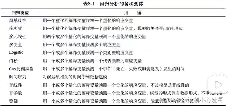
线性回归:普通最小二乘回归法(OLS)
类似于求解一元一次或一元多次方程

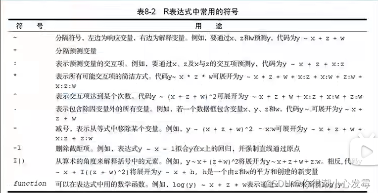
R表达式中常用的符号:
#------------------------------------------------------------#
# Chapter 49                                                 #
#------------------------------------------------------------#
ls("package:graphics")
help(package=graphics)
plot (women$height)
plot(women$height,women$weight)
plot(as.factor(women$height))
plot(mtcars$cyl)
plot(as.factor(mtcars$cyl))
plot(as.factor(mtcars$cyl),mtcars$carb)
plot(as.factor(mtcars$carb),as.factor(mtcars$cyl))
plot (women$height~ women$weight)
fit <- lm(height~ weight,data=women)
plot(fit)
methods(plot)
par()
?par
plot(as.factor(mtcars$cyl),col=c("red","green","blue"))


#------------------------------------------------------------#
# Chapter 50                                                 #
#------------------------------------------------------------#

mystats <- function(x,na.omit=FALSE) {
  if(na.omit)
    x <- x[!is.na(x)]
  m <- mean(x)
  n <- length(x)
  s <- sd(x)
  skew <- sum((x-m^3/s^3))/n
  kurt <- sum((x-m^4/s^4))/n-3
  return(c(n=n,mean=m,stdev=s,skew=skew,kurtosis=kurt))
 }

for (i in 1:10) {print ("Hello,World")}
#for ($i=1;$i<=10;$++) {print "hello,world\n";}
i=1;while(i <= 10) {print ("Hello,World");i=i+1;}
i=1;while(i <= 10) {print ("Hello,World");i=i+2;}
score=70;if (score >60 ) {print ("Passwd") } else {print ("Failed")}
ifelse( score >60,print ("Passwd"),print ("Failed"))

#switch
centre <- function(x, type) {
  switch(type,
         mean = mean(x),
         median = median(x),
         trimmed = mean(x, trim = .1))
}
x <- rcauchy(10)
centre(x, "mean")
centre(x, "median")
centre(x, "trimmed")
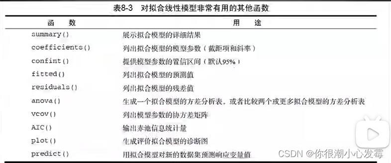
线性拟合常用函数:
#------------------------------------------------------------#
# Chapter 52                                                 #
#------------------------------------------------------------#
women
?lm
fit <- lm(weight ~ height, data=women)
summary(fit)
women$weight
fitted(fit)


#------------------------------------------------------------#
# Chapter 53                                                 #
#------------------------------------------------------------#
fit <- lm(weight ~ height, data=women)
coefficients(fit)
women$weight-fitted(fit)
residuals(fit)
women1 <- head(women,6)
predict(fit,women1)
plot(women$height,women$weight,
     main="Women Age 30-39",
     xlab="Height (in inches)",
     ylab="Weight (in pounds)")
# add the line of best fit
abline(fit)

#fit2
fit2 <- lm(weight ~ height + I(height^2), data=women)
summary(fit2)
summary(fit)
plot(women$height,women$weight,
     main="Women Age 30-39",
     xlab="Height (in inches)",
     ylab="Weight (in lbs)")
lines(women$height,fitted(fit2))
abline(fit)
lines(women$height,fitted(fit2),col="red")

# fit3
fit3 <- lm (weight~ height+I(height^2)+I(height^3),data=women)
plot(women$height,women$weight)
lines(women$height,fitted(fit))
lines(women$height,fitted(fit2),col="red")
lines(women$height,fitted(fit3),col="blue")
十、logistic回归模型代码
logistic回归模型,主要介绍使用R语言构建logistic回归模型用于分类问题的相关内容,内容包括数据读取与整理,模型构建,格式化输出,使用模型进行预测,使用ROC、AUC、混淆矩阵评估模型预测性能等。
# logistic回归
# 读取数据
bcdata <- read.csv(file.choose())

# 查看数据概况
library(skimr)
skim(bcdata)

# 删除含有缺失值的样本
bcdata <- na.omit(bcdata)

# 变量类型修正
bcdata$class <- factor(bcdata$class)

# 查看分类型变量编码
contrasts(bcdata$class)
# 查看分类型变量频数分布
table(bcdata$class)

# logistic回归建模
glmfit <- glm(class ~ .-ID, data = bcdata, family = binomial())
glmfit
summary(glmfit)

# 格式化输出
library(stargazer)
# 在console显示表格,输出到本地
stargazer(glmfit, type="text", out="logit.htm")

# 预测概率
predprob <- predict(glmfit, newdata = bcdata, type = "response")
# 有些模型的predict输出的概率是矩阵,注意识别。

# ROC曲线
library(pROC)
rocs <- roc(response = bcdata$class, # 实际类别
            predictor = predprob) # 预测概率
# 注意Setting direction

# ROC曲线
plot(
  rocs, # roc对象
  print.auc = TRUE, # 打印AUC值
  auc.polygon = TRUE, # 显示AUC区域
  grid = T, # 网格线
  max.auc.polygon = T, # 显示AUC=1的区域
  auc.polygon.col = "skyblue", # AUC区域填充色
  print.thres = T, # 打印最佳临界点
  legacy.axes = T # 横轴显示为1-specificity
)

# 约登法则
bestp <- rocs$thresholds[
  which.max(rocs$sensitivities + rocs$specificities - 1)
]
bestp

# 预测分类
predlab <- as.factor(
  ifelse(predprob > bestp, "malignant", "benign")
)

# 混淆矩阵
library(caret)
confusionMatrix(data = predlab, # 预测类别
                reference = bcdata$class, # 实际类别
                positive = "malignant",
                mode = "everything")
十一、数据分析实战
11.1多元线性回归
#------------------------------------------------------------#
# Chapter 54                                                 #
#------------------------------------------------------------#
states <- as.data.frame(state.x77[,c("Murder", "Population",
                                     "Illiteracy", "Income", "Frost")])
fit <- lm(Murder ~ Population + Illiteracy + Income + Frost, data=states)
summary(fit)
coef(fit)
qqPlot(fit, labels=row.names(states), id.method="identify",
       simulate=TRUE, main="Q-Q Plot")


# Mutiple linear regression with a significant interaction term
fit <- lm(mpg ~ hp + wt + hp:wt, data=mtcars)
summary(fit)

library(effects)
plot(effect("hp:wt", fit,, list(wt=c(2.2, 3.2, 4.2))), multiline=TRUE)

# AIC
fit1 <- lm (Murder ~ Population+Illiteracy+Income+Frost,data=states)
fit2 <- lm (Murder ~ Population+Illiteracy,data=states)
AIC(fit1,fit2)

# Backward stepwise selection
library(MASS)
states <- as.data.frame(state.x77[,c("Murder", "Population",
                                     "Illiteracy", "Income", "Frost")])
fit <- lm(Murder ~ Population + Illiteracy + Income + Frost,
          data=states)
stepAIC(fit, direction="backward")


#  All subsets regression
library(leaps)
states <- as.data.frame(state.x77[,c("Murder", "Population",
                                     "Illiteracy", "Income", "Frost")])
leaps <-regsubsets(Murder ~ Population + Illiteracy + Income +
                     Frost, data=states, nbest=4)
plot(leaps, scale="adjr2")
11.2回归诊断
这个模型是否是最佳模型?
模型多大程度满足OLS模型的统计假设?
模型是否经得起更多数据的检验?
如果拟合出来的模型指标不好,该如何继续下去?
满足OLS模型统计假设:
1、正态性:对于固定的自变量值,因变量值成正态分布
2、独立性:因变量之间互相独立
3、线性:因变量与自变量之间为线性相关
4、同方差性:因变量的方差不随自变量的水平不同而变化。也可称作不变方差
抽样法验证:

#------------------------------------------------------------#
# Chapter 55                                                 #
#------------------------------------------------------------#
opar <- par(no.readonly=TRUE)
fit <- lm(weight ~ height, data=women)
par(mfrow=c(2,2))
plot(fit)
par(opar)

fit2 <- lm(weight ~ height + I(height^2), data=women)
opar <- par(no.readonly=TRUE)
par(mfrow=c(2,2))
plot(fit2)
par(opar)

#------------------------------------------------------------#
# Chapter 56                                                 #
#------------------------------------------------------------#
?aov
11.3方差分析

R中因子的应用:
计算频数
独立性检验
相关性检验
方差分析
主成分分析
因子分析…
方差分析的应用:方差分析会大量应用在科学研究中,例如实验设计时,进行分组比较,例如药物研究实验,处理组与对照组进行比较。
方差分析有:
单因素方差分析ANOVA(组内,组间)
双因素方差分析ANOVA
协方差分析ANCOVA:即包含了协变量
多元方差分析MANOVA:即方差研究中包含多个因变量
多元协方差分析MANCOVA:即多元方差分析中存在协变量
#------------------------------------------------------------#
# Chapter 57                                                 #
#------------------------------------------------------------#
library(multcomp)
attach(cholesterol)
table(trt)
aggregate(response, by=list(trt), FUN=mean)
#aggregate(response, by=list(trt), FUN=sd)
fit <- aov(response ~ trt,data =cholesterol )
summary(fit)
fit.lm <- lm(response~trt,data=cholesterol)

# One-way ANCOVA
data(litter, package="multcomp")
attach(litter)
table(dose)
aggregate(weight, by=list(dose), FUN=mean)
fit <- aov(weight ~ gesttime + dose)
summary(fit)

# Two way ANOVA
attach(ToothGrowth)
table(supp,dose)
aggregate(len, by=list(supp,dose), FUN=mean)
aggregate(len, by=list(supp,dose), FUN=sd)
class(ToothGrowth$dose)
dose <- factor(dose)
fit <- aov(len~ supp*dose,data=ToothGrowth)
summary(fit)

install.packages("HH")
library(HH)
interaction.plot(dose, supp, len, type="b",
                 col=c("red","blue"), pch=c(16, 18),
                 main = "Interaction between Dose and Supplement Type")

# One-way MANOVA
library(MASS)
attach(UScereal)
shelf <- factor(shelf)
y <- cbind(calories, fat, sugars)
aggregate(y, by=list(shelf), FUN=mean)
cov(y)
fit <- manova(y ~ shelf)
summary(fit)
summary.aov(fit)
11.4功效分析

功效分析函数:
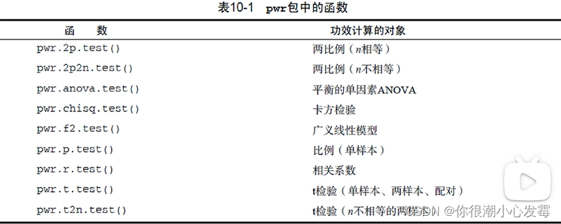
功效分析理论基础:

#------------------------------------------------------------#
# Chapter 58                                                 #
#------------------------------------------------------------#
install.packages("pwr")
library(pwr)

# Linear Models
pwr.f2.test(u=3, f2=0.0769, sig.level=0.05, power=0.90)
# ANOVA
pwr.anova.test(k=2,f=.25,sig.level=.05,power=.9)
# t tests
pwr.t.test(d=.8, sig.level=.05,power=.9, type="two.sample",
           alternative="two.sided")
pwr.t.test(n=20, d=.5, sig.level=.01, type="two.sample",
           alternative="two.sided")
# Correlations
pwr.r.test(r=.25, sig.level=.05, power=.90, alternative="greater")

# Tests of proportions
pwr.2p.test(h=ES.h(.65, .6), sig.level=.05, power=.9,
            alternative="greater")
# Chi-square tests
prob <- matrix(c(.42, .28, .03, .07, .10, .10), byrow=TRUE, nrow=3)
ES.w2(prob)
pwr.chisq.test(w=.1853, df=3 , sig.level=.05, power=.9)
11.5广义线性模型
线性回归和方差分析都是基于正态分布的假设,广义线性模型扩展了线性模型的框架,它包含了非正态因变量的分析。
泊松回归:
是用来为计数资料和列联表建模的一种回归分析。泊松回归假设因变量是泊松分布,并假设它平均值的对数可被未知参数的线性组合建模。
#------------------------------------------------------------#
# Chapter 59                                                 #
#------------------------------------------------------------#
?glm
data(breslow.dat, package="robust")
names(breslow.dat)
summary(breslow.dat[c(6, 7, 8, 10)])

attach(breslow.dat)
# fit regression
fit <- glm(sumY ~ Base + Age + Trt, data=breslow.dat, family=poisson(link="log"))
summary(fit)

# interpret model parameters
coef(fit)
exp(coef(fit))
11.6Logistic回归
当通过一系列连续型或类别型预测变量来预测二值型结果变量时,Logistic回归是一个非常有用的工具。
Logistic回归案例:

#------------------------------------------------------------#
# Chapter 60                                                 #
#------------------------------------------------------------#
data(Affairs, package="AER")
summary(Affairs)
table(Affairs$affairs)
prop.table(table(Affairs$affairs))
prop.table(table(Affairs$gender))

# create binary outcome variable
Affairs$ynaffair[Affairs$affairs > 0] <- 1
Affairs$ynaffair[Affairs$affairs == 0] <- 0
Affairs$ynaffair <- factor(Affairs$ynaffair,
                           levels=c(0,1),
                           labels=c("No","Yes"))
table(Affairs$ynaffair)

# fit full model
attach(Affairs)
fit <- glm(ynaffair ~ gender + age + yearsmarried + children +
                  religiousness + education + occupation +rating,
                data=Affairs,family=binomial())
summary(fit)

# fit reduced model
fit1 <- glm(ynaffair ~ age + yearsmarried + religiousness +
                     rating, data=Affairs, family=binomial())
summary(fit1)

# compare models
anova(fit, fit1, test="Chisq")

# interpret coefficients
coef(fit1)
exp(coef(fit1))

# calculate probability of extramariatal affair by marital ratings
testdata <- data.frame(rating = c(1, 2, 3, 4, 5),
                       age = mean(Affairs$age),
                       yearsmarried = mean(Affairs$yearsmarried),
                       religiousness = mean(Affairs$religiousness))
testdata$prob <- predict(fit1, newdata=testdata, type="response")
testdata

# calculate probabilites of extramariatal affair by age
testdata <- data.frame(rating = mean(Affairs$rating),
                       age = seq(17, 57, 10),
                       yearsmarried = mean(Affairs$yearsmarried),
                       religiousness = mean(Affairs$religiousness))
testdata$prob <- predict(fit1, newdata=testdata, type="response")
testdata
11.7主成分分析


#------------------------------------------------------------#
# Chapter 61                                                 #
#------------------------------------------------------------#
# Principal components analysis of US Judge Ratings
library(psych)
USJudgeRatings
fa.parallel(USJudgeRatings,fa="pc",n.iter = 100)
pc <- principal(USJudgeRatings, nfactors=1)
pc

# Principal components analysis Score
pc <- principal(USJudgeRatings,nfactors = 1,scores = TRUE)
pc$scores

# Principal components analysis Harman23.cor data
fa.parallel(Harman23.cor$cov, n.obs=302, fa="pc", n.iter=100,
            show.legend=FALSE, main="Scree plot with parallel analysis")

#Principal components analysis of body measurements
library(psych)
PC <- principal(Harman23.cor$cov, nfactors=2, rotate="none")
PC

#Principal components analysis with varimax rotation
rc <- principal(Harman23.cor$cov, nfactors=2, rotate="varimax")
rc
11.8因子分析


主成分与因子分析比较:


#------------------------------------------------------------#
# Chapter 62                                                 #
#------------------------------------------------------------#

options(digits=2)
library(psych)
covariances <- ability.cov$cov
# convert covariances to correlations
correlations <- cov2cor(covariances)
correlations

# determine number of factors to extract
fa.parallel(correlations, n.obs=112, fa="both", n.iter=100,
            main="Scree plots with parallel analysis")


# Principal axis factoring without rotation
fa <- fa(correlations, nfactors=2, rotate="none", fm="pa")
fa


# Factor extraction with orthogonal rotation
fa.varimax <- fa(correlations, nfactors=2, rotate="varimax", fm="pa")
fa.varimax


# Listing Factor extraction with oblique rotation
fa.promax <- fa(correlations, nfactors=2, rotate="promax", fm="pa")
fa.promax

# plot factor solution
factor.plot(fa.promax, labels=rownames(fa.promax$loadings))
fa.diagram(fa.promax, simple=FALSE)

# factor scores
fa <- fa(correlations,nfactors=2,rotate="none",fm="pa",score=TRUE)
fa.promax$weights
11.9购物篮分析
#------------------------------------------------------------#
# Chapter 63                                                 #
#------------------------------------------------------------#
install.packages("arules")
library(arules)
data(Groceries)
Groceries
inspect(Groceries)
fit <- apriori(Groceries,parameter = list(support=0.01,confidence=0.5))
summary(fit)
inspect(fit)
十二、R内置数据集
向量
euro #欧元汇率,长度为11,每个元素都有命名
landmasses #48个陆地的面积,每个都有命名
precip #长度为70的命名向量
rivers #北美141条河流长度
state.abb #美国50个州的双字母缩写
state.area #美国50个州的面积
state.name #美国50个州的全称
因子
state.division #美国50个州的分类,9个类别
state.region #美国50个州的地理分类
矩阵、数组
euro.cross #11种货币的汇率矩阵
freeny.x #每个季度影响收入四个因素的记录
state.x77 #美国50个州的八个指标
USPersonalExpenditure #5个年份在5个消费方向的数据
VADeaths #1940年弗吉尼亚州死亡率(每千人)
volcano #某火山区的地理信息(10米×10米的网格)
WorldPhones #8个区域在7个年份的电话总数
iris3 #3种鸢尾花形态数据
Titanic #泰坦尼克乘员统计
UCBAdmissions #伯克利分校1973年院系、录取和性别的频数
crimtab #3000个男性罪犯左手中指长度和身高关系
HairEyeColor #592人头发颜色、眼睛颜色和性别的频数
occupationalStatus #英国男性父子职业联系
类矩阵
eurodist #欧洲12个城市的距离矩阵,只有下三角部分
Harman23.cor #305个女孩八个形态指标的相关系数矩阵
Harman74.cor #145个儿童24个心理指标的相关系数矩阵
数据框
airquality #纽约1973年5-9月每日空气质量
anscombe #四组x-y数据,虽有相似的统计量,但实际数据差别较大
attenu #多个观测站对加利福尼亚23次地震的观测数据
attitude #30个部门在七个方面的调查结果,调查结果是同一部门35个职员赞成的百分比
beaver1 #一只海狸每10分钟的体温数据,共114条数据
beaver2 #另一只海狸每10分钟的体温数据,共100条数据
BOD #随水质的提高,生化反应对氧的需求(mg/l)随时间(天)的变化
cars #1920年代汽车速度对刹车距离的影响
chickwts #不同饮食种类对小鸡生长速度的影响
esoph #法国的一个食管癌病例对照研究
faithful #一个间歇泉的爆发时间和持续时间
Formaldehyde #两种方法测定甲醛浓度时分光光度计的读数
Freeny #每季度收入和其他四因素的记录
dating from #配对的病例对照数据,用于条件logistic回归
InsectSprays #使用不同杀虫剂时昆虫数目
iris #3种鸢尾花形态数据
LifeCycleSavings #50个国家的存款率
longley #强共线性的宏观经济数据
morley #光速测量试验数据
mtcars #32辆汽车在11个指标上的数据
OrchardSprays #使用拉丁方设计研究不同喷雾剂对蜜蜂的影响
PlantGrowth #三种处理方式对植物产量的影响
pressure #温度和气压
Puromycin #两种细胞中辅因子浓度对酶促反应的影响
quakes #1000次地震观测数据(震级>4)
randu #在VMS1.5中使用FORTRAN中的RANDU三个一组生成随机数字,共400组。
#该随机数字有问题。在VMS2.0以上版本已修复。
rock #48块石头的形态数据
sleep #两药物的催眠效果
stackloss #化工厂将氨转为硝酸的数据
swiss #瑞士生育率和社会经济指标
ToothGrowth #VC剂量和摄入方式对豚鼠牙齿的影响
trees #树木形态指标
USArrests #美国50个州的四个犯罪率指标
USJudgeRatings #43名律师的12个评价指标
warpbreaks #织布机异常数据
women #15名女性的身高和体重
列表
state.center #美国50个州中心的经度和纬度
类数据框
ChickWeight #饮食对鸡生长的影响
CO2 #耐寒植物CO2摄取的差异
DNase #若干次试验中,DNase浓度和光密度的关系
Indometh #某药物的药物动力学数据
Loblolly #火炬松的高度、年龄和种源
Orange #桔子树生长数据
Theoph #茶碱药动学数据
时间序列数据
airmiles #美国1937-1960年客运里程营收(实际售出机位乘以飞行哩数)
AirPassengers #Box &Jenkins航空公司1949-1960年每月国际航线乘客数
austres #澳大利亚1971-1994每季度人口数(以千为单位)
BJsales #有关销售的一个时间序列
BJsales.lead #前一指标的先行指标(leading indicator)
co2 #1959-1997年每月大气co2浓度(ppm)
discoveries #1860-1959年每年巨大发现或发明的个数
ldeaths #1974-1979年英国每月支气管炎、肺气肿和哮喘的死亡率
fdeaths #前述死亡率的女性部分
mdeaths #前述死亡率的男性部分
freeny.y #每季度收入
JohnsonJohnson #1960-1980年每季度Johnson &Johnson股票的红利
LakeHuron #1875-1972年某一湖泊水位的记录
lh #黄体生成素水平,10分钟测量一次
lynx #1821-1934年加拿大猞猁数据
nhtemp #1912-1971年每年平均温度
Nile #1871-1970尼罗河流量
nottem #1920-1939每月大气温度
presidents #1945-1974年每季度美国总统支持率
UKDriverDeaths #1969-1984年每月英国司机死亡或严重伤害的数目
sunspot.month #1749-1997每月太阳黑子数
sunspot.year #1700-1988每年太阳黑子数
sunspots #1749-1983每月太阳黑子数
treering #归一化的树木年轮数据
UKgas #1960-1986每月英国天然气消耗
USAccDeaths #1973-1978美国每月意外死亡人数
uspop #1790–1970美国每十年一次的人口总数(百万为单位)
WWWusage #每分钟网络连接数
Seatbelts #多变量时间序列。和UKDriverDeaths时间段相同,反映更多因素。
EuStockMarkets #多变量时间序列。欧洲股市四个主要指标的每个工作日记录。
总结
学习R语言的难点:
1.R是统计软件,会涉及到非常多统计学相关的内容;
2.软件的使用是通过在终端敲命令完成的;
3.每一部分内容都需要深入研究学习。


 2605
2605


 被折叠的 条评论
为什么被折叠?
被折叠的 条评论
为什么被折叠?
 到【灌水乐园】发言


