神经网络基础及逻辑回归实现

神经网络基础及逻辑回归实现

1. Logistic回归

1.1 Logistic回归

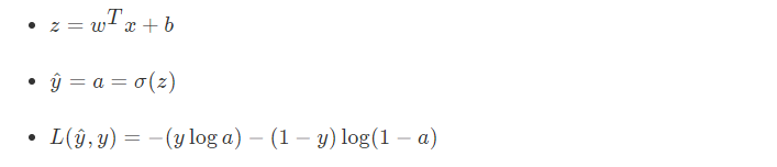
逻辑回归是一个主要用于二分分类类的算法。逻辑回归是给定一个x , 输出一个该样本属于1对应类别的预测概率​​=P(y=1∣x)。

Logistic 回归中使用的参数如下：

例如：

【这儿最后把逻辑回归结果和真实结果做对比】

1.2 逻辑回归损失函数

损失函数（loss function）用于衡量预测结果与真实值之间的误差。最简单的损失函数定义方式为平方差损失：

1.3 梯度下降算法

目的：使损失函数的值找到最小值

方式：梯度下降

函数的梯度（gradient）指出了函数的最陡增长方向。梯度的方向走，函数增长得就越快。那么按梯度的负方向走，函数值自然就降低得最快了。模型的训练目标即是寻找合适的 w 与 b 以最小化代价函数值。假设 w 与 b 都是一维实数，那么可以得到如下的 J 关于 w 与 b 的图：

可以看到，成本函数 J 是一个凸函数，与非凸函数的区别在于其不含有多个局部最低。

参数w和b的更新公式为：

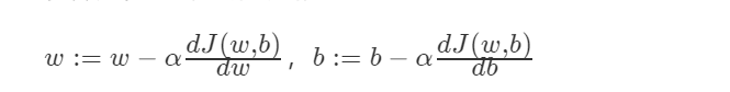
注：其中 α 表示学习速率，即每次更新的 w 的步伐长度。当 w 大于最优解 w′ 时，导数大于 0，那么 w 就会向更小的方向更新。反之当 w 小于最优解 w′ 时，导数小于 0，那么 w 就会向更大的方向更新。迭代直到收敛。

通过平面来理解梯度下降过程：

1.4 导数

理解梯度下降的过程之后，通过例子来说明梯度下降在计算导数意义或者说这个导数的意义。

1.4.1 导数

导数也可以理解成某一点处的斜率。斜率这个词更直观一些。

• 各点处的导数值一样

我们看到这里有一条直线，这条直线的斜率为4。我们来计算一个例子

例：取一点为a=2,那么y的值为8，我们稍微增加a的值为a=2.001,那么y的值为8.004，也就是当a增加了0.001，随后y增加了0.004，即4倍

那么我们的这个斜率可以理解为当一个点偏移一个不可估量的小的值，所增加的为4倍。

• 各点的导数值不全一致

例：取一点为a=2,那么y的值为4，我们稍微增加a的值为a=2.001,那么y的值约等于4.004（4.004001），也就是当a增加了0.001，随后y增加了4倍

取一点为a=5,那么y的值为25，我们稍微增加a的值为a=5.001,那么y的值约等于25.01（25.010001），也就是当a增加了0.001，随后y增加了10倍

可以得出该函数的导数2为2a。

• 更多函数的导数结果

1.4.2 导数计算图

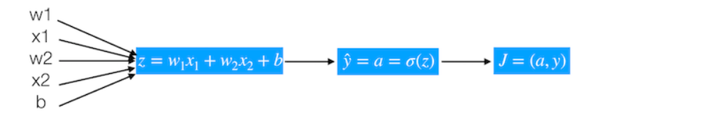
那么接下来我们来看看含有多个变量的到导数流程图，假设J(a,b,c)=3(a+bc)

我们以下面的流程图代替

这样就相当于从左到右计算出结果，然后从后往前计算出导数

• 导数计算

问题：那么现在我们要计算J相对于三个变量a,b,c的导数？

1.4.3 链式法则

1.4.4 逻辑回归的梯度下降

逻辑回归的梯度下降过程计算图，首先从前往后的计算图得出如下

那么计算图从前向过程为,假设样本有两个特征

问题：计算出J 关于z的导数

1.5 向量化编程

每更新一次梯度时候，在训练期间我们会拥有m个样本，那么这样每个样本提供进去都可以做一个梯度下降计算。所以我们要去做在所有样本上的计算结果、梯度等操作

1.5.1 向量化优势

什么是向量化

由于在进行计算的时候，最好不要使用for循环去进行计算，因为有Numpy可以进行更加快速的向量化计算。

在公式中w,x 都可能是多个值，也就是

import numpy as np
import time
a = np.random.rand(100000)
b = np.random.rand(100000)

• 第一种方法

# 第一种for 循环
c = 0
start = time.time()
for i in range(100000):
    c += a[i]*b[i]
end = time.time()

print("计算所用时间%s " % str(1000*(end-start)) + "ms")

• 第二种向量化方式使用np.dot

# 向量化运算
start = time.time()
c = np.dot(a, b)
end = time.time()
print("计算所用时间%s " % str(1000*(end-start)) + "ms")

执行效果：

关于Numpy中矩阵运算，具体详情查看博文：https://blog.csdn.net/weixin_44799217/article/details/113854203

Numpy能够充分的利用并行化，Numpy当中提供了很多函数使用

函数	作用
np.ones or np.zeros	全为1或者0的矩阵
np.exp	指数计算
np.log	对数计算
np.abs	绝对值计算

所以上述的m个样本的梯度更新过程，就是去除掉for循环。原本这样的计算

1.5.2 向量化实现伪代码

• 思路

可以变成这样的计算

注：w的形状为(n,1), x的形状为(n, m)，其中n为特征数量，m为样本数量

我们可以让，得出的结果为(1, m)大小的矩阵 注：大写的wx为多个样本表示

• 实现多个样本向量化计算的伪代码

这相当于一次使用了M个样本的所有特征值与目标值，那我们知道如果想多次迭代，使得这M个样本重复若干次计算

1.6 案例：实现逻辑回归

1.6.1使用数据：制作二分类数据集

from sklearn.datasets import load_iris, make_classification
from sklearn.model_selection import train_test_split
import tensorflow as tf
import numpy as np

X, Y = make_classification(n_samples=500, n_features=5, n_classes=2)
x_train, x_test, y_train, y_test = train_test_split(X, Y, test_size=0.3)

1.6.2 步骤设计：

分别构建算法的不同模块

• 1、初始化参数

def initialize_with_zeros(shape):
    """
    创建一个形状为 (shape, 1) 的w参数和b=0.
    return:w, b
    """

    w = np.zeros((shape, 1))
    b = 0

    return w, b

• 计算成本函数及其梯度
  • w (n,1).T * x (n, m)
  • y: (1, n)

def propagate(w, b, X, Y):
    """
    参数：w,b,X,Y：网络参数和数据
    Return:
    损失cost、参数W的梯度dw、参数b的梯度db
    """
    m = X.shape[1]

    # w (n,1), x (n, m)
    A = basic_sigmoid(np.dot(w.T, X) + b)
    # 计算损失
    cost = -1 / m * np.sum(Y * np.log(A) + (1 - Y) * np.log(1 - A))
    dz = A - Y
    dw = 1 / m * np.dot(X, dz.T)
    db = 1 / m * np.sum(dz)

    cost = np.squeeze(cost)

    grads = {"dw": dw,
             "db": db}

    return grads, cost

需要一个基础函数sigmoid

def basic_sigmoid(x):
    """
    计算sigmoid函数
    """

    s = 1 / (1 + np.exp(-x))

    return s

• 使用优化算法（梯度下降）
  • 实现优化函数. 全局的参数随着w,b对损失J进行优化改变. 对参数进行梯度下降公式计算，指定学习率和步长。
  • 循环：
    • 计算当前损失
    • 计算当前梯度
    • 更新参数（梯度下降）

def optimize(w, b, X, Y, num_iterations, learning_rate):
    """
    参数：
    w:权重,b:偏置,X特征,Y目标值,num_iterations总迭代次数,learning_rate学习率
    Returns:
    params:更新后的参数字典
    grads:梯度
    costs:损失结果
    """

    costs = []

    for i in range(num_iterations):

        # 梯度更新计算函数
        grads, cost = propagate(w, b, X, Y)

        # 取出两个部分参数的梯度
        dw = grads['dw']
        db = grads['db']

        # 按照梯度下降公式去计算
        w = w - learning_rate * dw
        b = b - learning_rate * db

        if i % 100 == 0:
            costs.append(cost)
        if i % 100 == 0:
            print("损失结果 %i: %f" %(i, cost))
            print(b)

    params = {"w": w,
              "b": b}

    grads = {"dw": dw,
             "db": db}

    return params, grads, costs

• 预测函数（不用实现）

利用得出的参数来进行测试得出准确率

def predict(w, b, X):
    '''
    利用训练好的参数预测
    return：预测结果
    '''

    m = X.shape[1]
    y_prediction = np.zeros((1, m))
    w = w.reshape(X.shape[0], 1)

    # 计算结果
    A = basic_sigmoid(np.dot(w.T, X) + b)

    for i in range(A.shape[1]):

        if A[0, i] <= 0.5:
            y_prediction[0, i] = 0
        else:
            y_prediction[0, i] = 1

    return y_prediction

• 整体逻辑
  • 模型训练

def model(x_train, y_train, x_test, y_test, num_iterations=2000, learning_rate=0.0001):
    """
    """

    # 修改数据形状
    x_train = x_train.reshape(-1, x_train.shape[0])
    x_test = x_test.reshape(-1, x_test.shape[0])
    y_train = y_train.reshape(1, y_train.shape[0])
    y_test = y_test.reshape(1, y_test.shape[0])
    print(x_train.shape)
    print(x_test.shape)
    print(y_train.shape)
    print(y_test.shape)

    # 1、初始化参数
    w, b = initialize_with_zeros(x_train.shape[0])

    # 2、梯度下降
    # params:更新后的网络参数
    # grads:最后一次梯度
    # costs:每次更新的损失列表
    params, grads, costs = optimize(w, b, x_train, y_train, num_iterations, learning_rate)

    # 获取训练的参数
    # 预测结果
    w = params['w']
    b = params['b']
    y_prediction_train = predict(w, b, x_train)
    y_prediction_test = predict(w, b, x_test)

    # 打印准确率
    print("训练集准确率: {} ".format(100 - np.mean(np.abs(y_prediction_train - y_train)) * 100))
    print("测试集准确率: {} ".format(100 - np.mean(np.abs(y_prediction_test - y_test)) * 100))

    return None

• 训练

model(x_train, y_train, x_test, y_test, num_iterations=2000, learning_rate=0.0001)

完整代码实现：

from sklearn.datasets import make_classification
from sklearn.model_selection import train_test_split
import numpy as np


X, Y = make_classification(n_samples=500, n_features=5, n_classes=2)
# print(X)
# print(Y)
x_train, x_test, y_train, y_test = train_test_split(X, Y, test_size=0.3)


#  初始化参数
def initialize_with_zero(shape):
    """
    创建一个形状为 (shape, 1) 的w参数和b=0.
    :param shape:
    :return:w,b
    """
    w = np.zeros((shape, 1))
    b = 0
    return w, b


#  sigmoid函数
def basic_sigmoid(x):
    """
    计算sigmoid函数
    :param x:
    :return:
    """
    s = 1 / (1 + np.exp(-x))

    return s


#  计算成本函数及其梯度
def propagate(w, b, X, Y):
    """
    参数：w,b,X,Y：网络参数和数据
    :return:
    损失cost、参数W的梯度dw、参数b的梯度db
    """
    m = X.shape[1]

    A = basic_sigmoid(np.dot(w.T, X) + b)

    #  计算损失
    cost = -1 / m * np.sum(Y * np.log(A) + (1 - Y) * np.log(1 - A))
    dz = A - Y
    dw = 1 / m * np.dot(X, dz.T)
    db = 1 / m * np.sum(dz)

    cost = np.squeeze(cost)

    grads = {'dw': dw, 'db': db}

    return grads, cost


#  优化算法（梯度下降）
def optimize(w, b, X, Y, num_iterations, learning_rate):
    """

    :param w: 权重
    :param b: 偏置
    :param X: 特征
    :param Y: 目标值
    :param num_iterations:迭代总次数
    :param learning_rate: 学习率
    :return:
    param:更新后的字典；grads：梯度；costs：损失结果
    """
    costs = []

    for i in range(num_iterations):
        #  梯度更新计算函数
        grads, cost = propagate(w, b, X, Y)

        #  取出两个部分参数的梯度
        dw = grads['dw']
        db = grads['db']

        #  按照梯度下降公式计算
        w = w - learning_rate * dw
        b = b - learning_rate * db

        if i % 100 == 0:
            costs.append(cost)
        if i % 100 == 0:
            print("损失结果 %i: %f" % (i, cost))
            print(b)

    params = {'w': w, 'b': b}
    grads = {'dw': dw, 'db': db}

    return params, grads, costs


#  预测函数
def predict(w, b, X):
    """
    利用训练好的参数预测
    :param w:
    :param b:
    :param X:
    :return: 预测结果
    """
    m = X.shape[1]
    y_prediction = np.zeros((1, m))
    w = w.reshape(X.shape[0], 1)

    #  计算结果
    A = basic_sigmoid(np.dot(w.T, X) + b)

    for i in range(A.shape[1]):
        if A[0, i] <= 0.5:
            y_prediction[0, i] = 0
        else:
            y_prediction[0, i] = 1

    return y_prediction


#  模型训练
def model(x_train, y_train, x_test, y_test, num_iterations=2000, learning_rate=0.0001):

    #  修改数据形状
    x_train = x_train.reshape(-1, x_train.shape[0])
    x_test = x_test.reshape(-1, x_test.shape[0])
    y_train = y_train.reshape(1, y_train.shape[0])
    y_test = y_test.reshape(1, y_test.shape[0])
    print(x_train.shape)
    print(x_test.shape)
    print(y_train.shape)
    print(y_test.shape)

    #  初始化参数
    w, b = initialize_with_zero(x_train.shape[0])

    #  梯度下降
    # params:更新后的网络参数
    # grads:最后一次梯度
    # costs:每次更新的损失列表
    params, grads, costs = optimize(w, b, x_train, y_train, num_iterations, learning_rate)

    #  获取训练的参数
    #  预测结果
    w = params['w']
    b = params['b']
    y_prediction_train = predict(w, b, x_train)
    y_prediction_test = predict(w, b, x_test)

    #  打印准确率
    print('训练集准确率：{}'.format(100 - np.mean(np.abs(y_prediction_train - y_train)) * 100))
    print("测试集准确率: {} ".format(100 - np.mean(np.abs(y_prediction_test - y_test)) * 100))

    return None


model(x_train, y_train, x_test, y_test, num_iterations=2000, learning_rate=0.0001)

运行结果：

(5, 350)
(5, 150)
(1, 350)
(1, 150)
损失结果 0: 0.693147
-2.285714285714286e-06
损失结果 100: 0.693125
-0.0002306037845439643
损失结果 200: 0.693104
-0.0004584208147545269
损失结果 300: 0.693082
-0.0006857377884934902
损失结果 400: 0.693061
-0.0009125556881695565
损失结果 500: 0.693040
-0.0011388754950187189
损失结果 600: 0.693019
-0.0013646981890990254
损失结果 700: 0.692998
-0.001590024749285418
损失结果 800: 0.692977
-0.0018148561532646467
损失结果 900: 0.692957
-0.0020391933775302648
损失结果 1000: 0.692936
-0.0022630373973777035
损失结果 1100: 0.692916
-0.0024863891868994077
损失结果 1200: 0.692896
-0.0027092497189800686
损失结果 1300: 0.692876
-0.00293161996529191
损失结果 1400: 0.692856
-0.003153500896290064
损失结果 1500: 0.692836
-0.003374893481207999
损失结果 1600: 0.692816
-0.003595798688053048
损失结果 1700: 0.692797
-0.0038162174836019807
损失结果 1800: 0.692777
-0.004036150833396662
损失结果 1900: 0.692758
-0.00425559970173978
训练集准确率：54.285714285714285
测试集准确率: 50.666666666666664