机器学习之逻辑回归与二分类

最新推荐文章于 2022-10-17 17:23:26 发布

weixin_44953902

最新推荐文章于 2022-10-17 17:23:26 发布

阅读量1.2k

点赞数 1

分类专栏：机器学习文章标签：机器学习逻辑回归 sklearn

本文链接：https://blog.csdn.net/weixin_44953902/article/details/96713439

版权

机器学习专栏收录该内容

18 篇文章 2 订阅

订阅专栏

分类算法–逻辑回归与二分类

逻辑回归（Logistic Regression）是机器学习中的一种分类模型，逻辑回归是一种分类算法，虽然名字中带有回归，但是它与回归之间有一定的联系。由于算法的简单和高效。在实际中应用非常广泛。

逻辑回归的应用场景

广告点击率
是否为垃圾邮件
是否患病
金融诈骗
虚假账号

从以上例子可以看出：它们都属于两个类别之间的判断。逻辑回归就是解决二分类问题的利器。

逻辑回归的原理

输入：

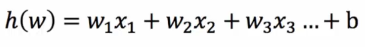
逻辑回归的输入就是一个线性回归的结果
在这里插入图片描述

激活函数

sigmoida函数：
$g(θ^Tx)=\frac{1}{1+e^{-θTx}}$
分析：
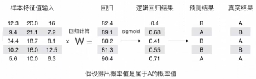
回归的结果输入到sigmoida函数当中
输出结果：[0,1]区间中的一个概率值，默认0.5为阈值
在这里插入图片描述

逻辑回归最终的分类是通过属于某个类别，并且这个类别默认标记为1（正例），另外的一个类别记为0（反例）。（损失计算）

输出结果解释：假设有两个类别A，B，并且假设概率值为1属于A类别。现有一个样本的输入到逻辑回归输出结果0.6，那么这个概率值超过0.5，意味着许小年连或者预测的结果就是A类别。那么反之，如果得出结果为0.3，那么，训练或者预测结果就是B类别。
在这里插入图片描述
之前线性回归预测结果使用均方误差来衡量，对于逻辑回归，使用什么来衡量预测结果的误差？

损失以及优化

损失
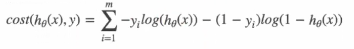
逻辑回归的损失，称为对数似然损失，公式如下：
按类别分开：

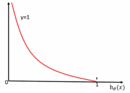
      当y=1时：即真实值为1，h(θ)得到的值为0时，从图中可以看出来，损失函数的值趋向于无穷，h(θ)得到的值为1时，损失函数的值趋向于0。

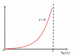
      当y=0时：即真实值为0，h(θ)得到的值为1时，从图中可以看出来，损失函数的值趋向于无穷，h(θ)得到的值为0时，损失函数的值趋向于0。

综合完整损失函数，

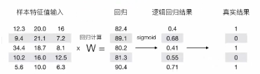
      计算损失：-（log(0.4)+(1-0)log(1-0.68)+log(0.41)+(1-0.55)log(1-0.55)+log(0.71)）
-log§：P值越大，损失越小。
优化
使用梯度下降法优化算法，去减少损失的值。这样去更新逻辑回归前面对应的算法的权重参数。

逻辑回归API

sklearn.linear_model LogisticRegression（solver='liblinear',penalty='l2',C=1.0）

solver：优化求解的方式（默认来源的liblinear库实现，内部使用了坐标轴下降法来迭代优化损失函数），sag：根据数据集来自动选择，随即平均梯度下降
penalty：正则化的种类
C：正则化力度
注：默认将类别数量少的当作正例。
LogisticRegression方法相当于SGDClassifier(loss=“log”,penalty=’ '),SGDClassifier实现了一个趋同的随机梯度下降学习，也支持平均随机梯度下降（ASGD），可以通过设置average=True。而使用LogisticRegression（实现了SAG）

案例：癌症分类预测-良/恶性乳腺肿瘤预测

流程分析：
（1）获取数据：读取的时候加上names
（2）数据处理：处理缺失值
（3）划分数据集
（4）特征工程：标准化
（5）逻辑回归预估器
（6）模型评估
代码：

import pandas as pd

import numpy as np

# 1.读取数据
path = "https://archive.ics.uci.edu/ml/machine-learning-databases/breast-cancer-wisconsin/breast-cancer-wisconsin.data"
column_name = ['Sample code number', 'Clump Thickness', 'Uniformity of Cell Size', 'Uniformity of Cell Shape',
               'Marginal Adhesion', 'Single Epithelial Cell Size', 'Bare Nuclei', 'Bland Chromatin',
               'Normal Nucleoli', 'Mitoses', 'Class']
data = pd.read_csv(path,names=column_name)

data.head()

	Sample code number	Clump Thickness	Uniformity of Cell Size	Uniformity of Cell Shape	Marginal Adhesion	Single Epithelial Cell Size	Bare Nuclei	Bland Chromatin	Normal Nucleoli	Mitoses	Class
0	1000025	5	1	1	1	2	1	3	1	1	2
1	1002945	5	4	4	5	7	10	3	2	1	2
2	1015425	3	1	1	1	2	2	3	1	1	2
3	1016277	6	8	8	1	3	4	3	7	1	2
4	1017023	4	1	1	3	2	1	3	1	1	2

# 2.缺失值处理
# 1)替换---->np.nan
data = data.replace(to_replace="?",value=np.nan)
# 2)缺失值处理（删除缺失样本）
data.dropna(inplace=True)

data.isnull().any()#不存在缺失值

Sample code number             False
Clump Thickness                False
Uniformity of Cell Size        False
Uniformity of Cell Shape       False
Marginal Adhesion              False
Single Epithelial Cell Size    False
Bare Nuclei                    False
Bland Chromatin                False
Normal Nucleoli                False
Mitoses                        False
Class                          False
dtype: bool

# 3.划分数据集
from sklearn.model_selection import train_test_split

# 筛选特征值和目标值
x = data.iloc[:,1:-1]
y = data["Class"]

x.head()

	Clump Thickness	Uniformity of Cell Size	Uniformity of Cell Shape	Marginal Adhesion	Single Epithelial Cell Size	Bare Nuclei	Bland Chromatin	Normal Nucleoli	Mitoses
0	5	1	1	1	2	1	3	1	1
1	5	4	4	5	7	10	3	2	1
2	3	1	1	1	2	2	3	1	1
3	6	8	8	1	3	4	3	7	1
4	4	1	1	3	2	1	3	1	1

x_train,x_test,y_train,y_test = train_test_split(x,y)

# 4.特征工程：标准化
from sklearn.preprocessing import StandardScaler

transfer = StandardScaler()
x_train = transfer.fit_transform(x_train)
x_test = transfer.transform(x_test)

x_train

array([[-0.86871961, -0.70102688, -0.74295671, ..., -0.17939874,
        -0.61860282, -0.36126301],
       [-0.86871961,  0.63949885, -0.05321267, ...,  1.46817358,
         0.68747819, -0.36126301],
       [-0.51599602,  1.30976171,  1.3262754 , ...,  0.23249434,
         1.66703895, -0.36126301],
       ...,
       [-0.16327244, -0.70102688, -0.74295671, ..., -1.00318491,
        -0.61860282, -0.36126301],
       [ 0.18945114, -0.70102688, -0.05321267, ..., -1.00318491,
        -0.61860282, -0.36126301],
       [-0.16327244, -0.70102688, -0.74295671, ..., -1.00318491,
        -0.61860282, -0.36126301]])

# 5.逻辑回归预估器
from sklearn.linear_model import LogisticRegression

estimator = LogisticRegression()
estimator.fit(x_train,y_train)

e:\python37\lib\site-packages\sklearn\linear_model\logistic.py:432: FutureWarning: Default solver will be changed to 'lbfgs' in 0.22. Specify a solver to silence this warning.
  FutureWarning)   
LogisticRegression(C=1.0, class_weight=None, dual=False, fit_intercept=True,
          intercept_scaling=1, max_iter=100, multi_class='warn',
          n_jobs=None, penalty='l2', random_state=None, solver='warn',
          tol=0.0001, verbose=0, warm_start=False)

# 逻辑回归模型参数：回归系数和偏置
estimator.coef_

array([[1.27684228, 0.39555928, 0.71283597, 0.74425675, 0.14041766,
        1.40653816, 1.04294598, 0.68242732, 0.85655016]])

estimator.intercept_

array([-0.9113462])

# 6.模型评估
y_predict = estimator.predict(x_test)
# 方法一：直接比对真实值和预测值
print("y_predict:\n",y_predict)
print("直接比对真实值和预测值：\n",y_test==y_predict)
# 方法二：计算准确率
score = estimator.score(x_test,y_test)
print("准确率为：\n",score)

y_predict:
 [4 4 2 4 2 4 4 2 2 2 4 2 4 2 2 2 2 2 4 4 2 4 2 4 2 2 2 2 2 2 4 4 2 2 2 2 2
 4 4 2 4 2 2 2 4 2 2 2 4 2 2 2 2 4 4 2 2 4 2 2 2 2 2 2 2 2 2 4 2 4 2 2 2 4
 2 2 2 4 4 4 2 4 4 2 2 4 2 2 2 2 4 2 2 4 4 2 2 2 4 2 4 4 4 2 2 2 4 2 2 4 2
 4 4 4 2 2 2 2 4 2 2 2 2 2 4 2 2 2 2 4 2 2 4 2 2 2 2 4 2 2 2 2 4 2 2 4 2 2
 2 4 2 2 2 4 4 2 2 2 2 4 2 2 2 4 2 4 2 4 2 4 2]
直接比对真实值和预测值：
 414     True
15      True
501     True
191     True
676     True
215     True
293     True
508     True
443     True
489    False
333     True
380     True
361     True
355     True
524     True
129     True
291     True
375     True
436     True
482     True
634     True
435     True
137     True
214     True
389     True
446     True
72      True
532     True
601     True
16      True
       ...  
347     True
295     True
671     True
486     True
434    False
181     True
66      True
348    False
570     True
392     True
492     True
502     True
262     True
173     True
462     True
307     True
572     True
395     True
230     True
341     True
37      True
557     True
479     True
624     True
132     True
265     True
681     True
463     True
142     True
209     True
Name: Class, Length: 171, dtype: bool
准确率为：
 0.9707602339181286

weixin_44953902

关注

1
点赞
踩
10

收藏

觉得还不错? 一键收藏
0
评论
机器学习之逻辑回归与二分类

分类算法–逻辑回归与二分类逻辑回归（Logistic Regression）是机器学习中的一种分类模型，逻辑回归是一种分类算法，虽然名字中带有回归，但是它与回归之间有一定的联系。由于算法的简单和高效。在实际中应用非常广泛。逻辑回归的应用场景广告点击率是否为垃圾邮件是否患病金融诈骗虚假账号从以上例子可以看出：它们都属于两个类别之间的判断。逻辑回归就是解决二分类问题的利器。逻辑回...
复制链接

扫一扫