利用python进行数据分析 第十四章 14.3 1880-2010年间全美婴儿姓名

14.3 1880-2010年间全美婴儿姓名

美国社会保障总署（SSA）ᨀ 供了一份从1880年到现在的婴儿名字频率数据。Hadley

Wickham（许多流行R包的作者）经常用这份数据来演示R的数据处理功能。

我们要做一些数据规整才能加载这个数据集，这么做就会产生一个如下的DataFrame：

In [4]: names.head(10)
Out[4]:
name sex births year
0 Mary F 7065 1880
1 Anna F 2604 1880
2 Emma F 2003 1880
3 Elizabeth F 1939 1880
4 Minnie F 1746 1880
5 Margaret F 1578 1880
6 Ida F 1472 1880
7 Alice F 1414 1880
8 Bertha F 1320 1880
9 Sarah F 1288 1880

你可以用这个数据集做很多事，例如：

计算指定名字（可以是你自己的，也可以是别人的）的年度比例。

计算Ḁ 个名字的相对排名。

计算各年度最流行的名字，以及增长或减少最快的名字。

分析名字趋势：元音、辅音、长度、总体多样性、拼写变化、首尾字母等。

分析外源性趋势：圣经中的名字、名人、人口结构变化等。

利用前面介绍过的那些工具，这些分析工作都能很轻松地完成，我会讲解其中的一些。

到编写本书时为止，美国社会保障总署将该数据库按年度制成了多个数据文件，其中给出了每个性

别/名字组合的出生总数。这些文件的原始档案可以在这里获

取： http://www.ssa.gov/oact/babynames/limits.html 。

如果你在阅读本书的时候这个页面已经不见了，也可以用搜索引擎找找。

下载"National data"文件names.zip，解压后的目录中含有一组文件（如yob1880.txt）。我用UNIX

的head命令查看了其中一个文件的前10行（在Windows上，你可以用more命令，或直接在文本编

辑器中打开）：

In [94]: !head -n 10 datasets/babynames/yob1880.txt
Mary,F,7065
Anna,F,2604
Emma,F,2003
Elizabeth,F,1939
Minnie,F,1746
Margaret,F,1578
Ida,F,1472
Alice,F,1414
Bertha,F,1320
Sarah,F,1288

由于这是一个非常标准的以逗号隔开的格式，所以可以用pandas.read_csv将其加载到DataFrame

中：

In [95]: import pandas as pd
In [96]: names1880 =
pd.read_csv('datasets/babynames/yob1880.txt',
....: names=['name', 'sex', 'births'])
In [97]: names1880
Out[97]:
name sex births
0 Mary F 7065
1 Anna F 2604
2 Emma F 2003
3 Elizabeth F 1939
4 Minnie F 1746
... ... .. ...
1995 Woodie M 5
1996 Worthy M 5
1997 Wright M 5
1998 York M 5
1999 Zachariah M 5
[2000 rows x 3 columns]

这些文件中仅含有当年出现超过5次的名字。为了简单起见，我们可以用births列的sex分组小计表

示该年度的births总计：

In [98]: names1880.groupby('sex').births.sum()
Out[98]:
sex
F 90993
M 110493
Name: births, dtype: int64

由于该数据集按年度被分隔成了多个文件，所以第一件事情就是要将所有数据都组装到一个

DataFrame里面，并加上一个year字段。使用pandas.concat即可达到这个目的：

years = range(1880, 2011)
pieces = []
columns = ['name', 'sex', 'births']
for year in years:
path = 'datasets/babynames/yob%d.txt' % year
frame = pd.read_csv(path, names=columns)
frame['year'] = year
pieces.append(frame)
# Concatenate everything into a single DataFrame
names = pd.concat(pieces, ignore_index=True)

这里需要注意几件事情。第一，concat默认是按行将多个DataFrame组合到一起的；第二，必须指

定ignore_index=True，因为我们不希望保留read_csv所返回的原始行号。现在我们得到了一个非

常大的DataFrame，它含有全部的名字数据：

In [100]: names
Out[100]:
name sex births year
0 Mary F 7065 1880
1 Anna F 2604 1880
2 Emma F 2003 1880
3 Elizabeth F 1939 1880
4 Minnie F 1746 1880
... ... .. ... ...
1690779 Zymaire M 5 2010
1690780 Zyonne M 5 2010
1690781 Zyquarius M 5 2010
1690782 Zyran M 5 2010
1690783 Zzyzx M 5 2010
[1690784 rows x 4 columns]

有了这些数据之后，我们就可以利用groupby或pivot_table在year和sex级别上对其进行聚合了，如

图14-4所示：

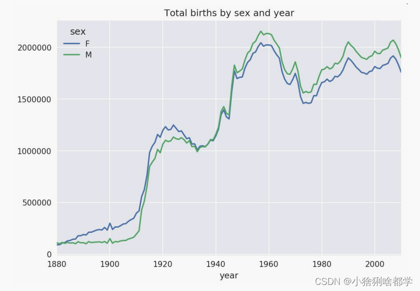
In [101]: total_births = names.pivot_table('births', index='year',
.....: columns='sex', aggfunc=sum)
In [102]: total_births.tail()
Out[102]:
425sex F M
year
2006 1896468 2050234
2007 1916888 2069242
2008 1883645 2032310
2009 1827643 1973359
2010 1759010 1898382
In [103]: total_births.plot(title='Total births by sex and year')

下面我们来插入一个prop列，用于存放指定名字的婴儿数相对于总出生数的比例。prop值为0.02表

示每100名婴儿中有2名取了当前这个名字。因此，我们先按year和sex分组，然后再将新列加到各

个分组上：

def add_prop(group):
group['prop'] = group.births / group.births.sum()
return group
names = names.groupby(['year', 'sex']).apply(add_prop)

现在，完整的数据集就有了下面这些列：

In [105]: names
Out[105]:
name sex births year prop
0 Mary F 7065 1880 0.077643
1 Anna F 2604 1880 0.028618
2 Emma F 2003 1880 0.022013
3 Elizabeth F 1939 1880 0.021309
4 Minnie F 1746 1880 0.019188
... ... .. ... ... ...
1690779 Zymaire M 5 2010 0.000003
1690780 Zyonne M 5 2010 0.000003
1690781 Zyquarius M 5 2010 0.000003
1690782 Zyran M 5 2010 0.000003
1690783 Zzyzx M 5 2010 0.000003
[1690784 rows x 5 columns]

在执行这样的分组处理时，一般都应该做一些有效性检查，比如验证所有分组的prop的总和是否为

1：

In [106]: names.groupby(['year', 'sex']).prop.sum()
Out[106]:
year sex
1880 F 1.0
M 1.0
1881 F 1.0
M 1.0
1882 F 1.0
...
2008 M 1.0
2009 F 1.0
M 1.0
2010 F 1.0
M 1.0
Name: prop, Length: 262, dtype: float64

工作完成。为了便于实现更进一步的分析，我需要取出该数据的一个子集：每对sex/year组合的前

1000个名字。这又是一个分组操作：

def get_top1000(group):
return group.sort_values(by='births', ascending=False)[:1000]
grouped = names.groupby(['year', 'sex'])
top1000 = grouped.apply(get_top1000)
# Drop the group index, not needed
top1000.reset_index(inplace=True, drop=True)

如果你喜欢DIY的话，也可以这样：

pieces = []
for year, group in names.groupby(['year', 'sex']):
pieces.append(group.sort_values(by='births', ascending=False)[:1000])
top1000 = pd.concat(pieces, ignore_index=True)

现在的结果数据集就小多了：

In [108]: top1000
Out[108]:
name sex births year prop
0 Mary F 7065 1880 0.077643
1 Anna F 2604 1880 0.028618
2 Emma F 2003 1880 0.022013
3 Elizabeth F 1939 1880 0.021309
4 Minnie F 1746 1880 0.019188
... ... .. ... ... ...
261872 Camilo M 194 2010 0.000102
261873 Destin M 194 2010 0.000102
261874 Jaquan M 194 2010 0.000102
261875 Jaydan M 194 2010 0.000102
261876 Maxton M 193 2010 0.000102
[261877 rows x 5 columns]

接下来的数据分析工作就针对这个top1000数据集了。

分析命名趋势

有了完整的数据集和刚才生成的top1000数据集，我们就可以开始分析各种命名趋势了。首先将前

1000个名字分为男女两个部分：

In [109]: boys = top1000[top1000.sex == 'M']
In [110]: girls = top1000[top1000.sex == 'F']

这是两个简单的时间序列，只需稍作整理即可绘制出相应的图表（比如每年叫做John和Mary的婴

儿数）。我们先生成一张按year和name统计的总出生数透视表：

In [111]: total_births = top1000.pivot_table('births', index='year',
.....: columns='name',
.....: aggfunc=sum)
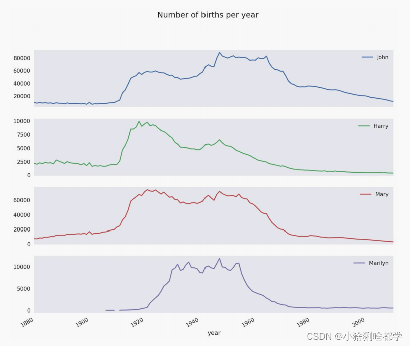
现在，我们用DataFrame的plot方法绘制几个名字的曲线图（见图14-5）：
In [112]: total_births.info()
<class 'pandas.core.frame.DataFrame'>
Int64Index: 131 entries, 1880 to 2010
Columns: 6868 entries, Aaden to Zuri
dtypes: float64(6868)
memory usage: 6.9 MB
In [113]: subset = total_births[['John', 'Harry', 'Mary', 'Marilyn']]
In [114]: subset.plot(subplots=True, figsize=(12, 10), grid=False,
.....: title="Number of births per year")

从图中可以看出，这几个名字在美国人民的心目中已经风光不再了。但事实并非如此简单，我们在

下一节中就能知道是怎么一回事了。

评估命名多样性的增长

一种解释是父母愿意给小孩起常见的名字越来越少。这个假设可以从数据中得到验证。一个办法是

计算最流行的1000个名字所占的比例，我按year和sex进行聚合并绘图（见图14-6）：

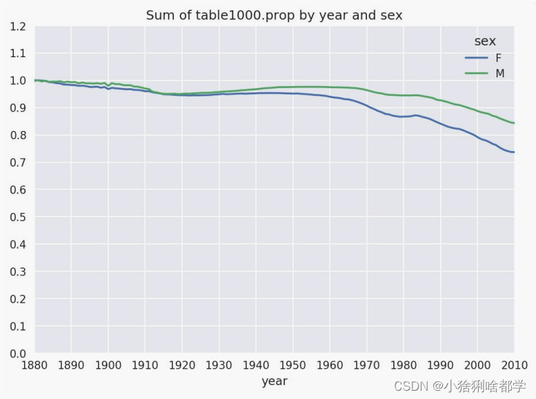
In [116]: table = top1000.pivot_table('prop', index='year',
.....: columns='sex', aggfunc=sum)
In [117]: table.plot(title='Sum of table1000.prop by year and sex',
.....: yticks=np.linspace(0, 1.2, 13), xticks=range(1880, 2020, 10)

从图中可以看出，名字的多样性确实出现了增长（前1000项的比例降低）。另一个办法是计算占

总出生人数前50%的不同名字的数量，这个数字不太好计算。我们只考虑2010年男孩的名字：

In [118]: df = boys[boys.year == 2010]
In [119]: df
Out[119]:
name sex births year prop
260877 Jacob M 21875 2010 0.011523
260878 Ethan M 17866 2010 0.009411
260879 Michael M 17133 2010 0.009025
260880 Jayden M 17030 2010 0.008971
260881 William M 16870 2010 0.008887
... ... .. ... ... ...
261872 Camilo M 194 2010 0.000102
261873 Destin M 194 2010 0.000102
261874 Jaquan M 194 2010 0.000102
261875 Jaydan M 194 2010 0.000102
261876 Maxton M 193 2010 0.000102
[1000 rows x 5 columns]

在对prop降序排列之后，我们想知道前面多少个名字的人数加起来才够50%。虽然编写一个for循

环确实也能达到目的，但NumPy有一种更聪明的矢量方式。先计算prop的累计和cumsum，然后

再通过searchsorted方法找出0.5应该被插入在哪个位置才能保证不破坏顺序：

In [120]: prop_cumsum = df.sort_values(by='prop', ascending=False).prop.cumsum()
In [121]: prop_cumsum[:10]
Out[121]:
260877 0.011523
260878 0.020934
260879 0.029959
260880 0.038930
260881 0.047817
260882 0.056579
260883 0.065155
260884 0.073414
260885 0.081528
260886 0.089621
Name: prop, dtype: float64
In [122]: prop_cumsum.values.searchsorted(0.5)
Out[122]: 116

由于数组索引是从0开始的，因此我们要给这个结果加1，即最终结果为117。拿1900年的数据来

做个比较，这个数字要小得多：

In [123]: df = boys[boys.year == 1900]
In [124]: in1900 = df.sort_values(by='prop', ascending=False).prop.cumsum()
In [125]: in1900.values.searchsorted(0.5) + 1
Out[125]: 25

现在就可以对所有year/sex组合执行这个计算了。按这两个字段进行groupby处理，然后用一个函

数计算各分组的这个值：

def get_quantile_count(group, q=0.5):
group = group.sort_values(by='prop', ascending=False)
return group.prop.cumsum().values.searchsorted(q) + 1
diversity = top1000.groupby(['year', 'sex']).apply(get_quantile_count)
diversity = diversity.unstack('sex')

现在，diversity这个DataFrame拥有两个时间序列（每个性别各一个，按年度索引）。通过

IPython，你可以查看其内容，还可以像之前那样绘制图表（如图14-7所示）：

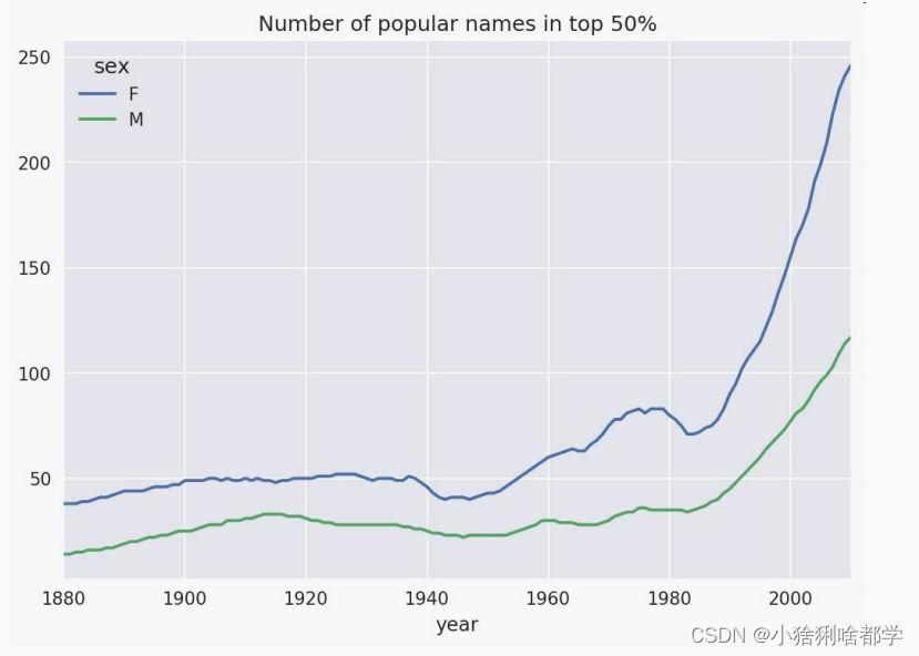
In [128]: diversity.head()
Out[128]:
sex F M
year
1880 38 14
1881 38 14
1882 38 15
1883 39 15
1884 39 16
In [129]: diversity.plot(title="Number of popular names in top 50%")

从图中可以看出，女孩名字的多样性总是比男孩的高，而且还在变得越来越高。读者们可以自己分

析一下具体是什么在驱动这个多样性（比如拼写形式的变化）。

“ 最后一个字母 ” 的变革

2007年，一名婴儿姓名研究人员Laura Wattenberg在她自己的网站上指出

（ http://www.babynamewizard.com）：近百年来，男孩名字在最后一个字母上的分布发生了显著

的变化。为了了解具体的情况，我首先将全部出生数据在年度、性别以及末字母上进行了聚合：

# extract last letter from name column

get_last_letter = lambda x: x[-1]
last_letters = names.name.map(get_last_letter)
last_letters.name = 'last_letter'
table = names.pivot_table('births', index=last_letters,
columns=['sex', 'year'], aggfunc=sum)

然后，我选出具有一定代表性的三年，并输出前面几行：

In [131]: subtable = table.reindex(columns=[1910, 1960, 2010], level='year')
In [132]: subtable.head()
Out[132]:
sex F M
year 1910 1960 2010 1910 1960 2010
last_letter
a 108376.0 691247.0 670605.0 977.0 5204.0 28438.0
b NaN 694.0 450.0 411.0 3912.0 38859.0
c 5.0 49.0 946.0 482.0 15476.0 23125.0
d 6750.0 3729.0 2607.0 22111.0 262112.0 44398.0
e 133569.0 435013.0 313833.0 28655.0 178823.0 129012.0

接下来我们需要按总出生数对该表进行规范化处理，以便计算出各性别各末字母占总出生人数的比

例：

In [133]: subtable.sum()
Out[133]:
sex year
F 1910 396416.0
1960 2022062.0
2010 1759010.0
M 1910 194198.0
1960 2132588.0
2010 1898382.0
dtype: float64
In [134]: letter_prop = subtable / subtable.sum()
In [135]: letter_prop
Out[135]:
sex F M
year 1910 1960 2010 1910 1960 2010
last_letter
a 0.273390 0.341853 0.381240 0.005031 0.002440 0.014980
b NaN 0.000343 0.000256 0.002116 0.001834 0.020470
c 0.000013 0.000024 0.000538 0.002482 0.007257 0.012181
d 0.017028 0.001844 0.001482 0.113858 0.122908 0.023387
e 0.336941 0.215133 0.178415 0.147556 0.083853 0.067959
... ... ... ... ... ... ...
v NaN 0.000060 0.000117 0.000113
0.000037 0.001434
w 0.000020 0.000031 0.001182 0.006329 0.007711 0.016148
x 0.000015 0.000037 0.000727 0.003965 0.001851 0.008614
y 0.110972 0.152569 0.116828 0.077349 0.160987 0.058168
z 0.002439 0.000659 0.000704 0.000170 0.000184 0.001831
[26 rows x 6 columns]

有了这个字母比例数据之后，就可以生成一张各年度各性别的条形图了，如图14-8所示：

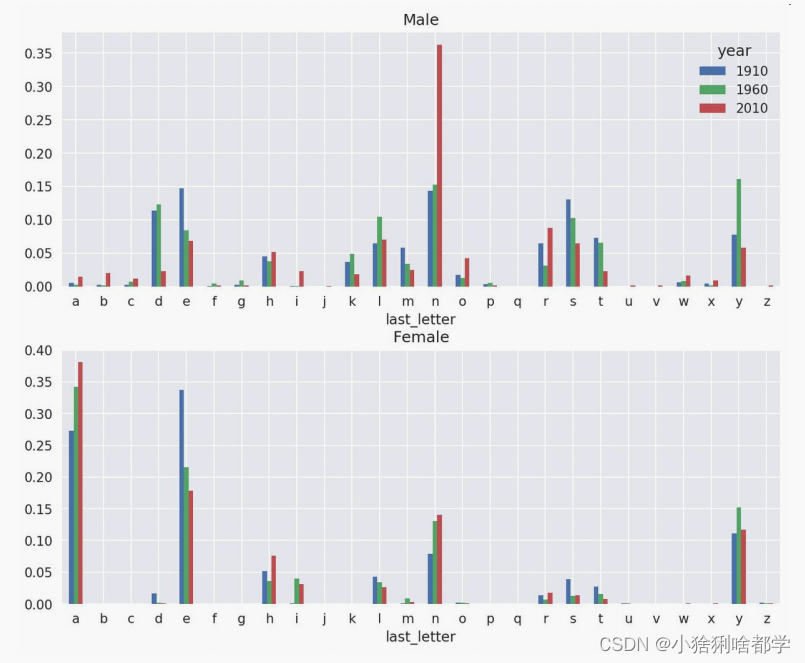
import matplotlib.pyplot as plt
fig, axes = plt.subplots(2, 1, figsize=(10, 8))
letter_prop['M'].plot(kind='bar', rot=0, ax=axes[0], title='Male')
letter_prop['F'].plot(kind='bar', rot=0, ax=axes[1], title='Female',
legend=False)

可以看出，从20世纪60年代开始，以字母"n"结尾的男孩名字出现了显著的增长。回到之前创建的

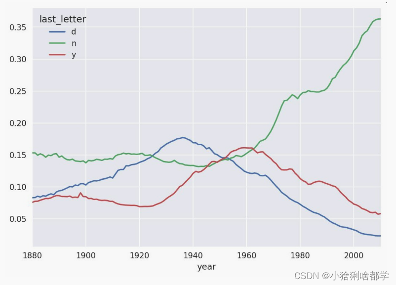
那个完整表，按年度和性别对其进行规范化处理，并在男孩名字中选取几个字母，最后进行转置以

便将各个列做成一个时间序列：

In [138]: letter_prop = table / table.sum()
In [139]: dny_ts = letter_prop.loc[['d', 'n', 'y'], 'M'].T
In [140]: dny_ts.head()
Out[140]:
last_letter d n y
year
1880 0.083055 0.153213 0.075760
1881 0.083247 0.153214 0.077451
1882 0.085340 0.149560 0.077537
1883 0.084066 0.151646 0.079144
1884 0.086120 0.149915 0.080405

有了这个时间序列的DataFrame之后，就可以通过其plot方法绘制出一张趋势图了（如图14-9所

示）：

In [143]: dny_ts.plot()

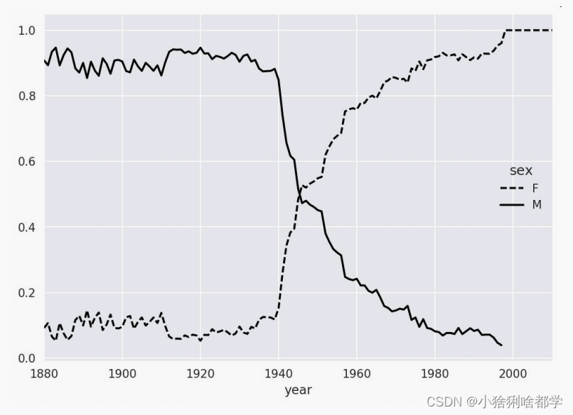
变成女孩名字的男孩名字（以及相反的情况）

另一个有趣的趋势是，早年流行于男孩的名字近年来“变性了”，例如Lesley或Leslie。回到top1000

数据集，找出其中以"lesl"开头的一组名字：

In [144]: all_names = pd.Series(top1000.name.unique())
In [145]: lesley_like = all_names[all_names.str.lower().str.contains('lesl')]
In [146]: lesley_like
Out[146]:
632 Leslie
2294 Lesley
4262 Leslee
4728 Lesli
6103 Lesly
dtype: object

然后利用这个结果过滤其他的名字，并按名字分组计算出生数以查看相对频率：

In [147]: filtered = top1000[top1000.name.isin(lesley_like)]
In [148]: filtered.groupby('name').births.sum()
Out[148]:
name
Leslee 1082
Lesley 35022
Lesli 929
Leslie 370429
Lesly 10067
Name: births, dtype: int64

接下来，我们按性别和年度进行聚合，并按年度进行规范化处理：

In [149]: table = filtered.pivot_table('births', index='year',
.....: columns='sex', aggfunc='sum')
In [150]: table = table.div(table.sum(1), axis=0)
In [151]: table.tail()
Out[151]:
sex F M
year
2006 1.0 NaN
2007 1.0 NaN
2008 1.0 NaN
2009 1.0 NaN
2010 1.0 NaN

最后，就可以轻松绘制一张分性别的年度曲线图了（如图2-10所示）：

In [153]: table.plot(style={'M': 'k-', 'F': 'k--'})

14.4 USDA食品数据库

美国农业部（USDA）制作了一份有关食物营养信息的数据库。Ashley Williams制作了该数据的

JSON版（ http://ashleyw.co.uk/project/food-nutrient-database）。其中的记录如下所示：

{
"id": 21441,
"description": "KENTUCKY FRIED CHICKEN, Fried Chicken, EXTRA CRISPY,
Wing, meat and skin with breading",
"tags": ["KFC"],
"manufacturer": "Kentucky Fried Chicken",
"group": "Fast Foods",
"portions": [
{
"amount": 1,
"unit": "wing, with skin",
"grams": 68.0
},
...
],
"nutrients": [
{
438"value": 20.8,
"units": "g",
"description": "Protein",
"group": "Composition"
},
...
]
}

每种食物都带有若干标识性属性以及两个有关营养成分和分量的列表。这种形式的数据不是很适合

分析工作，因此我们需要做一些规整化以使其具有更好用的形式。

从上面列举的那个网址下载并解压数据之后，你可以用任何喜欢的JSON库将其加载到Python中。

我用的是Python内置的json模块：

In [154]: import json
In [155]: db = json.load(open('datasets/usda_food/database.json'))
In [156]: len(db)
Out[156]: 6636

db中的每个条目都是一个含有Ḁ 种食物全部数据的字典。nutrients字段是一个字典列表，其中的每

个字典对应一种营养成分：

In [157]: db[0].keys()
Out[157]: dict_keys(['id', 'description', 'tags', 'manufacturer', 'group', 'porti
ons', 'nutrients'])
In [158]: db[0]['nutrients'][0]
Out[158]:
{'description': 'Protein',
'group': 'Composition',
'units': 'g',
'value': 25.18}
In [159]: nutrients = pd.DataFrame(db[0]['nutrients'])
In [160]: nutrients[:7]
Out[160]:
description group units value
0 Protein Composition g 25.18
1 Total lipid (fat) Composition g 29.20
2 Carbohydrate, by difference Composition g 3.06
3 Ash Other g 3.28
4 Energy Energy kcal 376.00
5 Water Composition g 39.28
6 Energy Energy kJ 1573.00

在将字典列表转换为DataFrame时，可以只抽取其中的一部分字段。这里，我们将取出食物的名

称、分类、编号以及制造商等信息：

In [161]: info_keys = ['description', 'group', 'id', 'manufacturer']
In [162]: info = pd.DataFrame(db, columns=info_keys)
In [163]: info[:5]
Out[163]:
description group id \
0 Cheese, caraway Dairy and Egg Products 1008
1 Cheese, cheddar Dairy and Egg Products 1009
2 Cheese, edam Dairy and Egg Products 1018
3 Cheese, feta Dairy and Egg Products 1019
4 Cheese, mozzarella, part skim milk Dairy and Egg Products 1028
manufacturer
0
1
2
3
4
In [164]: info.info()
<class 'pandas.core.frame.DataFrame'>
RangeIndex: 6636 entries, 0 to 6635
Data columns (total 4 columns):
description 6636 non-null object
group 6636 non-null object
id 6636 non-null int64
manufacturer 5195 non-null object
dtypes: int64(1), object(3)
memory usage: 207.5+ KB

通过value_counts，你可以查看食物类别的分布情况：

In [165]: pd.value_counts(info.group)[:10]
Out[165]:
Vegetables and Vegetable Products 812
Beef Products 618
Baked Products 496
Breakfast Cereals 403
Fast Foods 365
Legumes and Legume Products 365
Lamb, Veal, and Game Products 345
440Sweets 341
Pork Products 328
Fruits and Fruit Juices 328
Name: group, dtype: int64

现在，为了对全部营养数据做一些分析，最简单的办法是将所有食物的营养成分整合到一个大表

中。我们分几个步骤来实现该目的。首先，将各食物的营养成分列表转换为一个DataFrame，并添

加一个表示编号的列，然后将该DataFrame添加到一个列表中。最后通过concat将这些东西连接起

来就可以了：

顺利的话，nutrients的结果是：

In [167]: nutrients
Out[167]:
description group units value id
0 Protein Composition g 25.180 1008
1 Total lipid (fat) Composition g 29.200 1008
2 Carbohydrate, by difference Composition g 3.060 1008
3 Ash Other g 3.280 1008
4 Energy Energy kcal 376.000 1008
... ... ...
... ... ...
389350 Vitamin B-12, added Vitamins mcg 0.000 43546
389351 Cholesterol Other mg 0.000 43546
389352 Fatty acids, total saturated Other g 0.072 43546
389353 Fatty acids, total monounsaturated Other g 0.028 43546
389354 Fatty acids, total polyunsaturated Other g 0.041 43546
[389355 rows x 5 columns]

我发现这个DataFrame中无论如何都会有一些重复项，所以直接丢弃就可以了：

In [168]: nutrients.duplicated().sum() # number of duplicates
Out[168]: 14179
In [169]: nutrients = nutrients.drop_duplicates()

由于两个DataFrame对象中都有"group"和"description"，所以为了明确到底谁是谁，我们需要对它

们进行重命名：

In [170]: col_mapping = {'description' : 'food',
.....: 'group' : 'fgroup'}
In [171]: info = info.rename(columns=col_mapping, copy=False)
In [172]: info.info()
<class 'pandas.core.frame.DataFrame'>
RangeIndex: 6636 entries, 0 to 6635
Data columns (total 4 columns):
food 6636 non-null object
fgroup 6636 non-null object
id 6636 non-null int64
manufacturer 5195 non-null object
dtypes: int64(1), object(3)
memory usage: 207.5+ KB
In [173]: col_mapping = {'description' : 'nutrient',
.....: 'group' : 'nutgroup'}
In [174]: nutrients = nutrients.rename(columns=col_mapping, copy=False)
In [175]: nutrients
Out[175]:
nutrient nutgroup units value id
0 Protein Composition g 25.180 1008
1 Total lipid (fat) Composition g 29.200 1008
2 Carbohydrate, by difference Composition g 3.060 1008
3 Ash Other g 3.280 1008
4 Energy Energy kcal 376.000 1008
... ... ... ... ... ...
389350 Vitamin B-12, added Vitamins mcg 0.000 43546
389351 Cholesterol Other mg 0.000 43546
389352 Fatty acids, total saturated Other g 0.072 43546
389353 Fatty acids, total monounsaturated Other g 0.028 43546
389354 Fatty acids, total polyunsaturated Other g 0.041 43546
[375176 rows x 5 columns]

做完这些，就可以将info跟nutrients合并起来：

In [176]: ndata = pd.merge(nutrients, info, on='id', how='outer')
In [177]: ndata.info()
<class 'pandas.core.frame.DataFrame'>
Int64Index: 375176 entries, 0 to 375175
Data columns (total 8 columns):
nutrient 375176 non-null object
nutgroup 375176 non-null object
units 375176 non-null object
value 375176 non-null float64
id 375176 non-null int64
food 375176 non-null object
fgroup 375176 non-null object
manufacturer 293054 non-null object
dtypes: float64(1), int64(1), object(6)
memory usage: 25.8+ MB
In [178]: ndata.iloc[30000]
Out[178]:
nutrient Glycine
nutgroup Amino Acids
units g
value 0.04
id 6158
food Soup, tomato bisque, canned, condensed
fgroup Soups, Sauces, and Gravies
manufacturer
Name: 30000, dtype: object

我们现在可以根据食物分类和营养类型画出一张中位值图（如图14-11所示）：

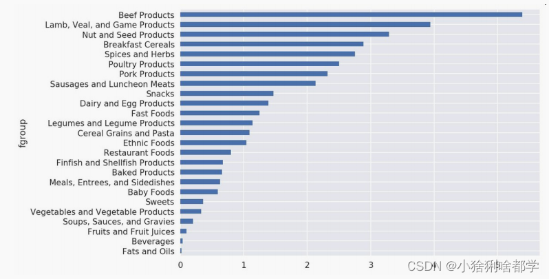
In [180]: result = ndata.groupby(['nutrient', 'fgroup'])['value'].quantile(0.5)
In [181]: result['Zinc, Zn'].sort_values().plot(kind='barh')

只要稍微动一动脑子，就可以发现各营养成分最为丰富的食物是什么了：

by_nutrient = ndata.groupby(['nutgroup', 'nutrient'])
get_maximum = lambda x: x.loc[x.value.idxmax()]
get_minimum = lambda x: x.loc[x.value.idxmin()]
max_foods = by_nutrient.apply(get_maximum)[['value', 'food']]
# make the food a little smaller
max_foods.food = max_foods.food.str[:50]

由于得到的DataFrame很大，所以不方便在书里面全部打印出来。这里只给出"Amino Acids"营养

分组：

In [183]: max_foods.loc['Amino Acids']['food']
Out[183]:
nutrient
Alanine Gelatins, dry powder, unsweetened
Arginine Seeds, sesame flour, low-fat
Aspartic acid Soy protein isolate
Cystine Seeds, cottonseed flour, low fat (glandless)
Glutamic acid Soy protein isolate
...
Serine Soy protein isolate, PROTEIN TECHNOLOGIES INTE...
Threonine Soy protein isolate, PROTEIN TECHNOLOGIES INTE...
Tryptophan Sea lion, Steller, meat with fat (Alaska Native)
Tyrosine Soy protein isolate, PROTEIN TECHNOLOGIES INTE...
Valine Soy protein isolate, PROTEIN TECHNOLOGIES INTE...
Name: food, Length: 19, dtype: object