机器学习十讲第四讲

模型误差的来源

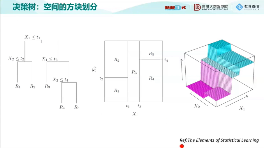
 决策树：空间的方块划分

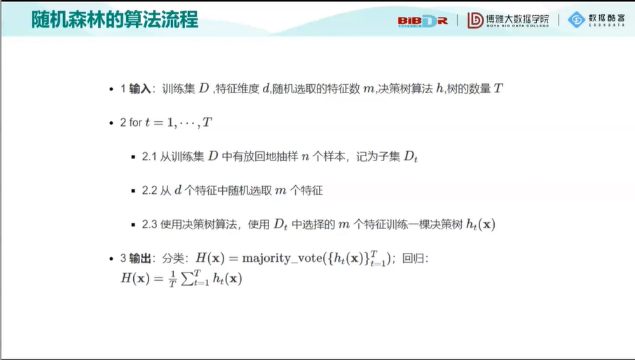
 随机森林：独立思考的重要性

决策树、随机森林和 AdaBoost 的 Python 实现

from sklearn.datasets import load_iris
import pandas as pd
import numpy as np
iris = load_iris()
iris_df = pd.DataFrame(data=iris.data,columns=iris.feature_names)
iris_df["target"] = iris.target
iris_df.head()
iris_df.columns = ["sepal_len","sepal_width","petal_len","petal_width","target"]
X_iris = iris_df.iloc[:,:-1]
y_iris = iris_df["target"]
#定义决策树节点
class TreeNode:
    def __init__(self, x_pos, y_pos, layer, class_labels=[0, 1, 2]):
        self.f = None  # 当前节点的切分特征
        self.v = None  # 当前节点的切分点
        self.left = None  # 左儿子节点
        self.right = None  # 右儿子节点
        self.pos = (x_pos, y_pos)  # 节点坐标，可视化用
        self.label_dist = None  # 当前节点样本的类分布
        self.layer = layer
        self.class_labels = class_labels
def __str__(self):  # 打印节点信息，可视化时的节点标签
    if self.f != None:
        return self.f + "\n<=" + str(round(self.v, 2))
    else:
        return str(self.label_dist) + "\n(" + str(np.sum(self.label_dist)) + ")"
#基尼系数计算
def gini(y):
    return 1 - np.square(y.value_counts()/len(y)).sum()
#分类决策树生成
def generate(X,y,x_pos,y_pos,nodes,min_leaf_samples,max_depth,layer,class_labels):
    current_node = TreeNode(x_pos,y_pos,layer,class_labels)#创建节点对象
    current_node.label_dist = [len(y[y==v]) for v in class_labels] #当前节点类样本分布
    nodes.append(current_node)
    if(len(X) < min_leaf_samples or gini(y) < 0.1 or layer > max_depth): #判断是否需要生成子节点
        return current_node
    max_gini,best_f,best_v = 0,None,None
    for f in X.columns: #特征遍历
        for v in X[f].unique(): #取值遍历
            y1,y2 = y[X[f] <= v],y[X[f] > v]
            if (len(y1) >= min_leaf_samples and len(y2) >= min_leaf_samples):
                imp_descent = gini(y) - gini(y1)*len(y1)/len(y) - gini(y2)*len(y2)/len(y) # 计算不纯度变化
                if imp_descent > max_gini:
                    max_gini,best_f,best_v = imp_descent,f,v
    current_node.f,current_node.v = best_f,best_v
    if(current_node.f != None):
        current_node.left = generate(X[X[best_f] <= best_v],y[X[best_f] <= best_v],x_pos-(2**(max_depth-layer)),y_pos -1,nodes,min_leaf_samples,max_depth,layer + 1,class_labels)
        current_node.right = generate(X[X[best_f] > best_v],y[X[best_f] > best_v],x_pos+ (2**(max_depth-layer)),y_pos -1,nodes,min_leaf_samples,max_depth,layer + 1,class_labels)
    return current_node
#输入为训练数据，叶子节点最小样本数和树的最大深度。返回树的根，节点集合。
def decision_tree_classifier(X,y,min_leaf_samples,max_depth):
    nodes = []
    root = generate(X,y,0,0,nodes,min_leaf_samples=min_leaf_samples,max_depth=max_depth,layer=1,class_labels=y.unique())
    return root,nodes
#使用 Networkx 将决策树可视化
def get_networkx_graph(G, root):
    if root.left != None:
        G.add_edge(root, root.left) #在当前节点和左儿子节点之间建立一条边，加入G
        get_networkx_graph(G, root.left) #对左儿子执行同样操作
    if root.right != None:
        G.add_edge(root, root.right) #在当前节点和左儿子节点之间建立一条边，加入G
        get_networkx_graph(G,root.right)#对右儿子执行同样操作
def get_tree_pos(G):
    pos = {}
    for node in G.nodes:
        pos[node] = node.pos
    return pos
def get_node_color(G):
    color_dict = []
    for node in G.nodes:
        if node.f == None:  #叶子节点
            label = np.argmax(node.label_dist)
            if label%3 == 0:
                color_dict.append("#007979") #深绿色
            elif label%3 == 1:
                color_dict.append("#E4007F") #洋红色
            else:
                color_dict.append("blue")
        else:
            color_dict.append("gray")
    return color_dict
import matplotlib.pyplot as plt
import networkx as nx
#1训练决策树
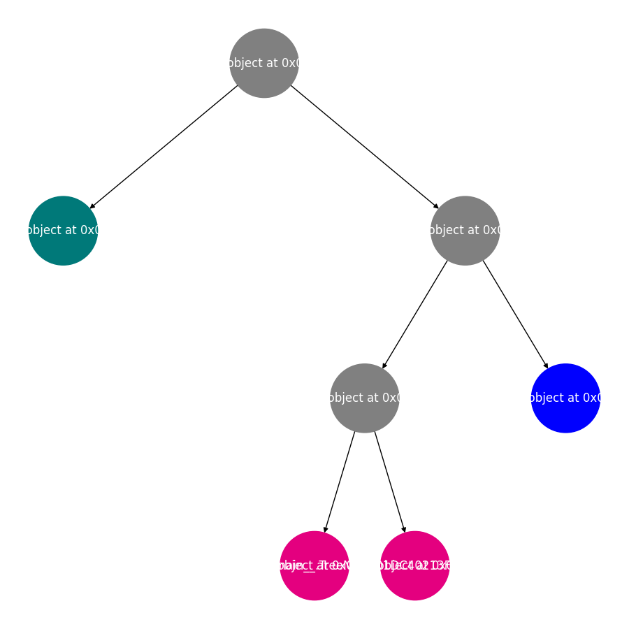
root,nodes = decision_tree_classifier(X_iris,y_iris,min_leaf_samples=10,max_depth=4)
#2将决策树进行可视化
fig, ax = plt.subplots(figsize=(9, 9)) #2.1将图的大小设置为 9×9
graph = nx.DiGraph() #2.2 创建 Networkx 中的网络对象
get_networkx_graph(graph, root) # 2.3 将决策树转换成 Networkx 的网络对象
pos = get_tree_pos(graph) #2.4 获取节点的坐标
# 2.5 绘制决策树
nx.draw_networkx(graph,pos = pos,ax = ax,node_shape="o",font_color="w",node_size=5000,node_color=get_node_color(graph))
plt.box(False) #去掉边框
plt.axis("off")#不显示坐标轴
plt.show()
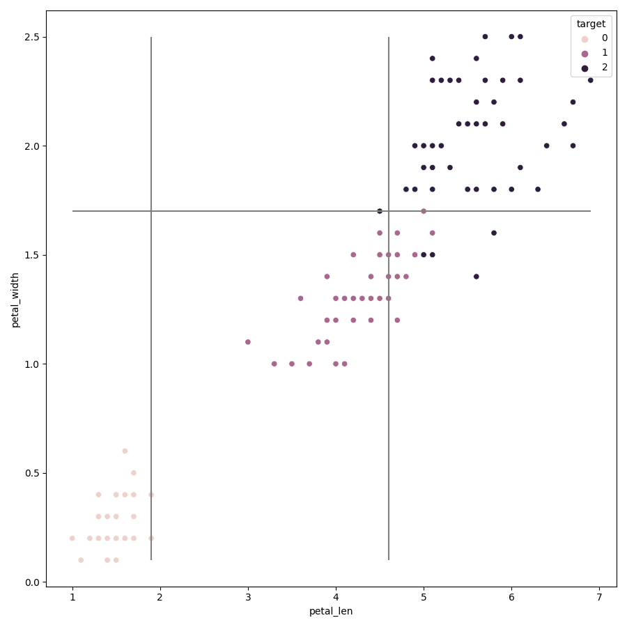
#决策树的决策边界
import seaborn as sns
#筛选两列特征
feature_names = ["petal_len","petal_width"]
X = iris_df[feature_names]
y = iris_df["target"]
#训练决策树模型
tree_two_dimension, nodes = decision_tree_classifier(X,y,min_leaf_samples=10,max_depth=4)
#开始绘制决策边界
fig, ax = plt.subplots(figsize=(9, 9)) #设置图片大小
sns.scatterplot(x = X.iloc[:,0], y = X.iloc[:,1],ax = ax,hue = y) #绘制样本点
#遍历决策树节点，绘制划分直线
for node in nodes:
    if node.f == X.columns[0]:
        ax.vlines(node.v,X.iloc[:,1].min(),X.iloc[:,1].max(),color="gray") # 如果节点分裂特征是 petal_len ，则绘制竖线
    elif node.f == X.columns[1]:
        ax.hlines(node.v,X.iloc[:,0].min(),X.iloc[:,0].max(),color="gray") #如果节点分裂特征是 petal_width ，则绘制水平线
#开始绘制决策边界
fig, ax = plt.subplots(figsize=(9, 9)) #设置图片大小
sns.scatterplot(x = X.iloc[:,0], y = X.iloc[:,1],ax = ax,hue = y) #绘制样本点
#遍历决策树节点，绘制划分直线
for node in nodes:
    if node.f == X.columns[0]:
        ax.vlines(node.v,X.iloc[:,1].min(),X.iloc[:,1].max(),color="gray") # 如果节点分裂特征是 petal_len ，则绘制竖线
    elif node.f == X.columns[1]:
        ax.hlines(node.v,X.iloc[:,0].min(),X.iloc[:,0].max(),color="gray") #如果节点分裂特征是 petal_width ，则绘制水平线


def plot_tree_boundary(X, y, tree, nodes):
    # 优化计算每个决策线段的起始点
    for node in nodes:
        node.x0_min, node.x0_max, node.x1_min, node.x1_max = X.iloc[:, 0].min(), X.iloc[:, 0].max(), X.iloc[:,1].min(), X.iloc[:,1].max(),
    node_list = []
    node_list.append(tree)
    while (len(node_list) > 0):
        node = node_list.pop()
        if node.f != None:
            node_list.append(node.left)
            node_list.append(node.right)
        if node.f == X.columns[0]:
            node.left.x0_max = node.v
            node.right.x0_min = node.v
        elif node.f == X.columns[1]:
            node.left.x1_max = node.v
            node.right.x1_min = node.v

    fig, ax = plt.subplots(figsize=(9, 9))  # 设置图片大小
    sns.scatterplot(x=X.iloc[:, 0], y=X.iloc[:, 1], ax=ax, hue=y)  # 绘制样本点
    # 遍历决策树节点，绘制划分直线
    for node in nodes:
        if node.f == X.columns[0]:
            ax.vlines(node.v, node.x1_min, node.x1_max, color="gray")  # 如果是节点分裂特征是 petal_len ，则绘制竖线
        elif node.f == X.columns[1]:
            ax.hlines(node.v, node.x0_min, node.x0_max, color="gray")  # 如果是节点分裂特征是 petal_width ，则绘制水平线
    # 绘制边框
    ax.vlines(X.iloc[:, 0].min(), X.iloc[:, 1].min(), X.iloc[:, 1].max(), color="gray")
    ax.vlines(X.iloc[:, 0].max(), X.iloc[:, 1].min(), X.iloc[:, 1].max(), color="gray")
    ax.hlines(X.iloc[:, 1].min(), X.iloc[:, 0].min(), X.iloc[:, 0].max(), color="gray")
    ax.hlines(X.iloc[:, 1].max(), X.iloc[:, 0].min(), X.iloc[:, 0].max(), color="gray")
    plt.show()
plot_tree_boundary(X,y,tree_two_dimension,nodes)