08.3. 语言模型和数据集

最新推荐文章于 2024-04-27 22:52:25 发布

nsq_ai

最新推荐文章于 2024-04-27 22:52:25 发布

阅读量1k

点赞数 4

分类专栏： Python基础学习 python书籍笔记 # dive_into_deep_learning 文章标签：语言模型人工智能自然语言处理

本文链接：https://blog.csdn.net/weixin_45063703/article/details/127221670

版权

Python基础学习同时被 3 个专栏收录

123 篇文章 17 订阅

订阅专栏

python书籍笔记

78 篇文章 4 订阅

订阅专栏

dive_into_deep_learning

69 篇文章 0 订阅

订阅专栏

文章目录

- 8.3. 语言模型和数据集

8.3. 语言模型和数据集

在给定这样的文本序列时，语言模型（language model）的目标是估计序列的联合概率.
一个理想的语言模型就能够基于模型本身生成自然文本。

8.3.1. 学习语言模型

我们面对的问题是如何对一个文档，甚至是一个词元序列进行建模。

为了训练语言模型，我们需要计算单词的概率，以及给定前面几个单词后出现某个单词的条件概率。
这些概率本质上就是语言模型的参数。

拉普拉斯平滑（Laplace smoothing），有助于处理单元素问题，是在所有计数中添加一个小常量。单词组合指定为非零计数，否则将无法在语言模型中使用它们。

8.3.2. 马尔可夫模型与n元语法

通常，涉及一个、两个和三个变量的概率公式分别被称为 “一元语法”（unigram）、“二元语法”（bigram）和“三元语法”（trigram）模型。

8.3.3. 自然语言统计

我们看看在真实数据上如果进行自然语言统计。
根据 8.2节中介绍的时光机器数据集构建词表，并打印前个最常用的（频率最高的）单词。

import random
import torch
from d2l import torch as d2l

tokens = d2l.tokenize(d2l.read_time_machine())
# 因为每个文本行不一定是一个句子或一个段落，因此我们把所有文本行拼接到一起
corpus = [token for line in tokens for token in line]
vocab = d2l.Vocab(corpus)
vocab.token_freqs[:10]

# result
[('the', 2261),
 ('i', 1267),
 ('and', 1245),
 ('of', 1155),
 ('a', 816),
 ('to', 695),
 ('was', 552),
 ('in', 541),
 ('that', 443),
 ('my', 440)]

正如我们所看到的，最流行的词看起来很无聊，这些词通常被称为停用词（stop words），因此可以被过滤掉。
尽管如此，它们本身仍然是有意义的，我们仍然会在模型中使用它们。
此外，还有个明显的问题是词频衰减的速度相当地快。

freqs = [freq for token, freq in vocab.token_freqs]
d2l.plot(freqs, xlabel='token: x', ylabel='frequency: n(x)',
        xscale='log', yscale='log')

在这里插入图片描述

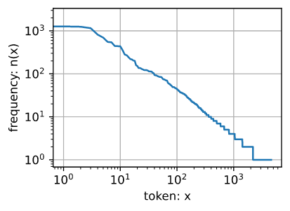
词频以一种明确的方式迅速衰减。
将前几个单词作为例外消除后，剩余的所有单词大致遵循双对数坐标图上的一条直线。

# 二元语法的频率
bigram_tokens = [pair for pair in zip(corpus[:-1], corpus[1:])]
bigram_vocab = d2l.Vocab(bigram_tokens)
bigram_vocab.token_freqs[:10]

#result
# 在十个最频繁的词对中，有九个是由两个停用词组成的， 只有一个与“the time”有关。
[(('of', 'the'), 309),
(('in', 'the'), 169),
(('i', 'had'), 130),
(('i', 'was'), 112),
(('and', 'the'), 109),
(('the', 'time'), 102),
(('it', 'was'), 99),
(('to', 'the'), 85),
(('as', 'i'), 78),
(('of', 'a'), 73)]

# 三元语法的频率
trigram_tokens = [triple for triple in zip(
   corpus[:-2], corpus[1:-1], corpus[2:])]
trigram_vocab = d2l.Vocab(trigram_tokens)
trigram_vocab.token_freqs[:10]


# result
[(('the', 'time', 'traveller'), 59),
(('the', 'time', 'machine'), 30),
(('the', 'medical', 'man'), 24),
(('it', 'seemed', 'to'), 16),
(('it', 'was', 'a'), 15),
(('here', 'and', 'there'), 15),
(('seemed', 'to', 'me'), 14),
(('i', 'did', 'not'), 14),
(('i', 'saw', 'the'), 13),
(('i', 'began', 'to'), 13)]

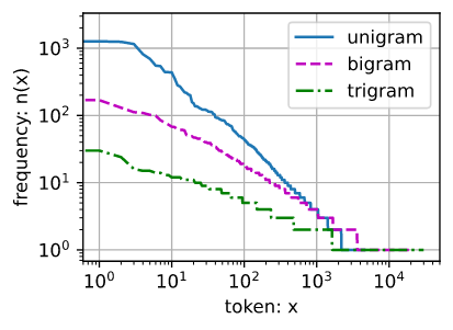
# 最后，我们直观地对比三种模型中的词元频率：一元语法、二元语法和三元语法。
bigram_freqs = [freq for token, freq in bigram_vocab.token_freqs]
trigram_freqs = [freq for token, freq in trigram_vocab.token_freqs]
d2l.plot([freqs, bigram_freqs, trigram_freqs], xlabel='token: x',
        ylabel='frequency: n(x)', xscale='log', yscale='log',
        legend=['unigram', 'bigram', 'trigram'])

在这里插入图片描述

8.3.4. 读取长序列数据

由于序列数据本质上是连续的，因此我们在处理数据时需要解决这个问题.

假设我们将使用神经网络来训练语言模型，模型中的网络一次处理具有预定义长度（例如个时间步）的一个小批量序列。
任意长的序列可以被我们划分为具有相同时间步数的子序列。
当训练我们的神经网络时，这样的小批量子序列将被输入到模型中。假设网络一次只处理具有个时间步的子序列
在这里插入图片描述

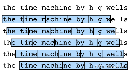
分割文本时，不同的偏移量会导致不同的子序列

如果我们只选择一个偏移量，那么用于训练网络的、所有可能的子序列的覆盖范围将是有限的.
因此，我们可以从随机偏移量开始划分序列，以同时获得覆盖性（coverage）和随机性（randomness）。

8.3.4.1. 随机采样

在随机采样中，每个样本都是在原始的长序列上任意捕获的子序列。
在迭代过程中，来自两个相邻的、随机的、小批量中的子序列不一定在原始序列上相邻。
对于语言建模，目标是基于到目前为止我们看到的词元来预测下一个词元，因此标签是移位了一个词元的原始序列。

参数batch_size指定了每个小批量中子序列样本的数目，参数num_steps是每个子序列中预定义的时间步数。

def seq_data_iter_random(corpus, batch_size, num_steps):  #@save
    """使用随机抽样生成一个小批量子序列"""
    # 从随机偏移量开始对序列进行分区，随机范围包括num_steps-1
    corpus = corpus[random.randint(0, num_steps - 1):]
    # 减去1，是因为我们需要考虑标签
    num_subseqs = (len(corpus) - 1) // num_steps
    # 长度为num_steps的子序列的起始索引
    initial_indices = list(range(0, num_subseqs * num_steps, num_steps))
    # 在随机抽样的迭代过程中，
    # 来自两个相邻的、随机的、小批量中的子序列不一定在原始序列上相邻
    random.shuffle(initial_indices)

    def data(pos):
        # 返回从pos位置开始的长度为num_steps的序列
        return corpus[pos: pos + num_steps]

    num_batches = num_subseqs // batch_size
    for i in range(0, batch_size * num_batches, batch_size):
        # 在这里，initial_indices包含子序列的随机起始索引
        initial_indices_per_batch = initial_indices[i: i + batch_size]
        X = [data(j) for j in initial_indices_per_batch]
        Y = [data(j + 1) for j in initial_indices_per_batch]
        yield torch.tensor(X), torch.tensor(Y)
        
# 生成一个从0到34的序列
my_seq = list(range(35))
for X, Y in seq_data_iter_random(my_seq, batch_size=2, num_steps=5):
    print('X: ', X, '\nY:', Y)

# result
X:  tensor([[14, 15, 16, 17, 18],
        [ 9, 10, 11, 12, 13]])
Y: tensor([[15, 16, 17, 18, 19],
        [10, 11, 12, 13, 14]])
X:  tensor([[19, 20, 21, 22, 23],
        [29, 30, 31, 32, 33]])
Y: tensor([[20, 21, 22, 23, 24],
        [30, 31, 32, 33, 34]])
X:  tensor([[ 4,  5,  6,  7,  8],
        [24, 25, 26, 27, 28]])
Y: tensor([[ 5,  6,  7,  8,  9],
        [25, 26, 27, 28, 29]])

8.3.4.2. 顺序分区

顺序分区:
保证两个相邻的小批量中的子序列在原始序列上也是相邻的,基于小批量的迭代过程中保留了拆分的子序列的顺序.

def seq_data_iter_sequential(corpus, batch_size, num_steps):  #@save
    """使用顺序分区生成一个小批量子序列"""
    # 从随机偏移量开始划分序列
    offset = random.randint(0, num_steps)
    num_tokens = ((len(corpus) - offset - 1) // batch_size) * batch_size
    Xs = torch.tensor(corpus[offset: offset + num_tokens])
    Ys = torch.tensor(corpus[offset + 1: offset + 1 + num_tokens])
    Xs, Ys = Xs.reshape(batch_size, -1), Ys.reshape(batch_size, -1)
    num_batches = Xs.shape[1] // num_steps
    for i in range(0, num_steps * num_batches, num_steps):
        X = Xs[:, i: i + num_steps]
        Y = Ys[:, i: i + num_steps]
        yield X, Y
# 基于相同的设置，通过顺序分区读取每个小批量的子序列的特征X和标签Y
for X, Y in seq_data_iter_sequential(my_seq, batch_size=2, num_steps=5):
    print('X: ', X, '\nY:', Y)
    
# result
X:  tensor([[ 4,  5,  6,  7,  8],
        [19, 20, 21, 22, 23]])
Y: tensor([[ 5,  6,  7,  8,  9],
        [20, 21, 22, 23, 24]])
X:  tensor([[ 9, 10, 11, 12, 13],
        [24, 25, 26, 27, 28]])
Y: tensor([[10, 11, 12, 13, 14],
        [25, 26, 27, 28, 29]])
X:  tensor([[14, 15, 16, 17, 18],
        [29, 30, 31, 32, 33]])
Y: tensor([[15, 16, 17, 18, 19],
        [30, 31, 32, 33, 34]])
        
# 现在，我们将上面的两个采样函数包装到一个类中， 以便稍后可以将其用作数据迭代器。
class SeqDataLoader:  #@save
    """加载序列数据的迭代器"""
    def __init__(self, batch_size, num_steps, use_random_iter, max_tokens):
        if use_random_iter:
            self.data_iter_fn = d2l.seq_data_iter_random
        else:
            self.data_iter_fn = d2l.seq_data_iter_sequential
        self.corpus, self.vocab = d2l.load_corpus_time_machine(max_tokens)
        self.batch_size, self.num_steps = batch_size, num_steps

    def __iter__(self):
        return self.data_iter_fn(self.corpus, self.batch_size, self.num_steps)

# 定义了一个函数load_data_time_machine， 它同时返回数据迭代器和词表， 因此可以与其他带有load_data前缀的函数 
def load_data_time_machine(batch_size, num_steps,  #@save
                           use_random_iter=False, max_tokens=10000):
    """返回时光机器数据集的迭代器和词表"""
    data_iter = SeqDataLoader(
        batch_size, num_steps, use_random_iter, max_tokens)
    return data_iter, data_iter.vocab

8.3.5. 小结

语言模型是自然语言处理的关键。
元语法通过截断相关性，为处理长序列提供了一种实用的模型。
长序列存在一个问题：它们很少出现或者从不出现。
齐普夫定律支配着单词的分布，这个分布不仅适用于一元语法，还适用于其他元语法。
通过拉普拉斯平滑法可以有效地处理结构丰富而频率不足的低频词词组。
读取长序列的主要方式是随机采样和顺序分区。在迭代过程中，后者可以保证来自两个相邻的小批量中的子序列在原始序列上也是相邻的

nsq_ai

关注

4
点赞
踩
9

收藏

觉得还不错? 一键收藏
打赏
3
评论
08.3. 语言模型和数据集

读取长序列的主要方式是随机采样和顺序分区。在迭代过程中，后者可以保证来自两个相邻的小批量中的子序列在原始序列上也是相邻的。假设我们将使用神经网络来训练语言模型，模型中的网络一次处理具有预定义长度（例如个时间步）的一个小批量序列。保证两个相邻的小批量中的子序列在原始序列上也是相邻的,基于小批量的迭代过程中保留了拆分的子序列的顺序.在给定这样的文本序列时，语言模型（language model）的目标是估计序列的联合概率.如果我们只选择一个偏移量，那么用于训练网络的、所有可能的子序列的覆盖范围将是有限的.
复制链接

扫一扫