机器学习—有监督学习—单变量线性回归(推导及代码实现)

一、算法推导

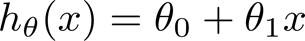
1、单变量线性回归模型

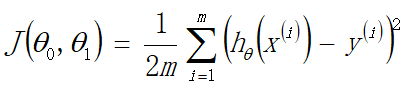
2、代价函数定义（误差平方和代价函数）

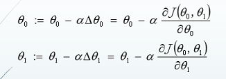
3、优化目标：寻找代价函数的最小值点（梯度下降算法）

梯度下降的关键是代价函数对参数θ0，θ1求偏导，找到梯度下降的方向。

通过参数更新方程，不断迭代，对参数θ通过学习率α，不断朝代价函数的最低点进行优化，最终迭代出最优参数。

二、简单线性回归—代码实现(数据集最后)

1、导库

import numpy as np
import matplotlib.pyplot as plt

2、读取数据

#可使用loadtxt()函数读取txt文档，delimiter=','代表以逗号分隔开
data = np.loadtxt('./data1.txt',delimiter=',')

#数据读取    最后一列前都为特征   最后一列为标签
X = data[:,:-1]
y = data[:,-1]

#数据初始化  方便矩阵操作
X = np.c_[np.ones(len(X)),X]
y = np.c_[y]

#还可以进行数据切分操作70%为训练集，30%为测试集(由于数据小,这里没有进行数据切分操作)

3、定义模型

def model(X,theta):
    h = np.dot(X,theta)
    return h

4、代价函数

#定义代价函数
def costFunc(h,y):
    m = y.shape[0]
    J = 1.0/(2*m)*np.sum(np.square(h-y))
    # J = 1.0/(2*m)*np.dot((h-y).T,(h-y))     两种代价函数表示形式
    return J

5、梯度下降算法

#定义梯度下降函数
def gradDesc(X,y,alpha=0.01,iter_num=2000):
    m,n = X.shape
    theta = np.zeros((n,1)) #初始化theta值
    J_history = np.zeros(iter_num) #初始化代价函数值

    #执行梯度下降
    for i in range(iter_num):
        h = model(X,theta)
        J_history[i] = costFunc(h,y)

        #参数迭代更新
        deltatheta = (1.0/m)*np.dot(X.T,h-y)
        theta -= alpha*deltatheta
    return J_history,theta

#调用梯度下降算法
J_history,theta = gradDesc(X,y)
print(theta)

6、画图

#画代价曲线
plt.title('代价曲线')
plt.plot(J_history)
plt.xlabel('迭代次数')
plt.ylabel('代价值')
plt.show()

#画样本散点图，和线性回归方程
#散点图
plt.scatter(X[:,1],y[:,0],c='r')

#画回归方程
min_x,max_x = np.min(X[:,1]),np.max(X[:,1])
min_x_y,max_x_y = theta[0]+theta[1]*min_x,theta[0]+theta[1]*max_x
plt.plot([min_x,max_x],[min_x_y,max_x_y])

plt.show()

7、线性模型评价指标—精度

#定义精度函数
#精度: 1-u/v,           u为误差的平方和,   v为真实结果 减 真实结果均值 的平方和
def score(h,y):
    u = np.sum(np.square(h-y))
    v = np.sum(np.square(y-np.mean(y)))
    score = 1-u/v
    return score
    
h = model(X,theta)
print('该模型精度为：',score(h,y))

----结果展示       精度约为95.6%，比较符合该数据集
该模型精度为： 0.9559231295276738

8、可视化展示

代价函数曲线(可用来调整参数大小)

三、学习完了单变量线性回归，多变量线性回归是在单变量线性回归的基础上增加了更多的特征，算法设计思路一致，下方超链接是对多变量线性回归的总结。

---

多变量线性回归算法的推导与代码实现

四、数据集

9.540,29.083
8.021,23.368
1.689,8.862
4.285,15.782
3.036,12.282
2.985,11.220
5.129,17.264
9.871,34.502
5.422,16.372
7.522,20.053
8.655,22.760
9.281,30.578
7.929,24.127
0.556,6.203
5.658,17.831
1.438,8.529
5.654,18.970
0.914,7.217
6.572,23.589
1.997,9.529
7.480,20.249
8.478,22.470
8.768,26.106
2.466,11.373
8.435,28.167
5.083,17.829
2.753,12.094
8.678,26.921
2.008,9.363
6.212,21.713
3.655,15.953
9.940,33.469
8.159,27.669
8.687,29.392
6.196,19.460
7.359,25.092
3.509,14.297
9.562,26.596
5.867,21.941
6.713,20.673
8.460,23.833
7.982,24.207
2.009,10.729
1.179,7.861
6.522,18.737
1.075,7.738
3.360,12.792
5.984,20.137
3.765,15.896
0.129,5.376
1.523,8.196
5.176,17.967
8.118,22.594
8.569,26.270
3.377,12.592
0.759,6.571
2.629,12.298
7.457,21.847
0.945,6.967
7.019,19.281
5.675,17.571
9.268,26.627
9.432,28.023
3.237,11.919
4.144,14.198
1.412,9.171
2.469,11.954
0.310,5.886
0.481,6.265
0.724,6.668
2.830,12.154
3.678,14.475
4.595,17.491
2.348,10.946
6.069,18.702
6.196,21.151
1.620,8.578
7.897,25.457
9.643,25.782
2.311,10.264
1.870,9.351
4.801,18.298
3.408,14.008
5.355,18.826
8.684,25.572
7.117,23.510
7.065,19.468
9.965,30.734
0.781,6.880
2.906,12.826
0.827,7.313
4.371,16.071
2.307,10.463
4.292,16.548
7.234,26.493
1.475,9.408
1.448,8.951
1.333,8.786
2.542,11.175
8.542,28.551