采用GDAL批量波段运算计算植被指数0基础教程

采用GDAL批量波段运算计算植被指数0基础教程

1. 引言

在传统的遥感数据处理方法中，通常使用ArcGis或ENVI软件进行波段运算。然而，这些软件在处理大量数据时往往效率低下。有没有一种方法可以批量进行波段运算，一下子计算几十个植被指数，并自动保存计算后的指标影像到相应目录下呢？答案是肯定的！本文将介绍如何使用GDAL库实现这一目标。

2. GDAL简介

GDAL（Geospatial Data Abstraction Library）是一个用于处理栅格数据和矢量数据的开源库，是地理信息系统（GIS）和遥感领域的重要工具之一。GDAL的详细介绍及其安装可以查看这篇文章：GDAL介绍及安装。

3. 植被指数计算公式

这里列出了要计算的23种植被指数及其计算公式：

• DVI 为差值植被指数；
• EVI 为增强植被指数；
• GCVI 为绿光归一化差值植被指数；
• GNDVI 为绿光归一化差值植被指数；
• ISR1, ISR2 为短波红外比值植被指数；
• LSWI 为地表水分指数；
• MSAVI 为修正型土壤调节植被指数；
• NDPI 为归一化差异物候指数；
• NDVI 为归一化植被指数；
• NDWI1, NDWI2, NDWI3 为归一化水体指数；
• RENDVI1, RENDVI2 为红边归一化差值植被指数；
• RENDWI1, RENDWI2 为红边归一化水体指数；
• SAVI 为土壤调节植被指数；
• SR 为比值植被指数；
• TR1, TR2 为比值生物学变量植被指数；
• VRE1, VRE2 为红边植被指数。

植被指数	计算公式
DVI	DVI = nir - red
EVI	EVI = 2.5 × (nir - red)/(nir + 6 × red - 7.5 × blue + 1)
GCVI	GCVI = nir/green - 1
GNDVI	GNDVI = (nir - green)/(nir + green)
ISR1	ISR1 = nir/swir1
ISR2	ISR2 = nir/swir2
LSWI	LSWI = (nir - swir1)/(nir + swir1)
MSAVI	MSAVI = 1/2 × (2 × nir + 1 - ((2 × nir + 1)^2 - 8 × (nir - red))^(1/2))
NDPI	NDPI = (nir - (0.74 × red + 0.26 × swir1))/(nir + (0.74 × red + 0.26 × swir1))
NDVI	NDVI = (nir - red)/(nir + red)
NDWI1	NDWI1 = (nir - swir1)/(nir + swir1)
NDWI2	NDWI2 = (nir - swir2)/(nir + swir2)
NDWI3	NDWI3 = (green - nir)/(green + nir)
RENDVI1	RENDVI1 = (nir - red1)/(nir + red1)
RENDVI2	RENDVI2 = (nir - red2)/(nir + red2)
RENDWI1	RENDWI1 = (red1 - swir1)/(red1 + swir1)
RENDWI2	RENDWI2 = (red2 - swir1)/(red2 + swir1)
SAVI	SAVI = (1 + L) × (nir - red)/(nir + red + 0.5)
SR	SR = nir/red
TR1	TR1 = (1/red1 - 1/red1) × nir
TR2	TR2 = (1/red - 1/nir) × red2
VRE1	VRE1 = nir/red1
VRE2	VRE2 = nir/red2

4. 批量计算植被指数

使用 gdal_calc.py 工具可以批量计算表格中各植被指数。以下是计算这些植被指数的命令示例：

python gdal_calc.py -A ronghe.tif --A_band=5 -B ronghe.tif --B_band=4 --outfile=dvi.tif --calc="A-B"

python gdal_calc.py -A ronghe.tif --A_band=5 -B ronghe.tif --B_band=4 -C ronghe.tif --C_band=2 --outfile=evi.tif --calc="2.5*((A-B)/(A+6*B-7.5*C+1))"

python gdal_calc.py -A ronghe.tif --A_band=5 -B ronghe.tif --B_band=3 --outfile=gcvi.tif --calc="(A/B)-1"

python gdal_calc.py -A ronghe.tif --A_band=5 -B ronghe.tif --B_band=3 --outfile=gndvi.tif --calc="(A-B)/(A+B)"

python gdal_calc.py -A ronghe.tif --A_band=5 -B ronghe.tif --B_band=6 --outfile=isr1.tif --calc="A/B"

python gdal_calc.py -A ronghe.tif --A_band=5 -B ronghe.tif --B_band=7 --outfile=isr2.tif --calc="A/B"

python gdal_calc.py -A ronghe.tif --A_band=5 -B ronghe.tif --B_band=6 --outfile=lswi.tif --calc="(A-B)/(A+B)"

python gdal_calc.py -A ronghe.tif --A_band=5 -B ronghe.tif --B_band=4 --outfile=msavi.tif --calc="0.5*(2*A+1-((2*A+1)**2-8*(A-B))**0.5)"

python gdal_calc.py -A ronghe.tif --A_band=5 -B ronghe.tif --B_band=4 -C ronghe.tif --C_band=6 --outfile=ndpi.tif --calc="(A-(0.74*B+0.26*C))/(A+(0.74*B+0.26*C))"

python gdal_calc.py -A ronghe.tif --A_band=5 -B ronghe.tif --B_band=4 --outfile=ndvi.tif --calc="(A-B)/(A+B)"

python gdal_calc.py -A ronghe.tif --A_band=5 -B ronghe.tif --B_band=6 --outfile=ndwi1.tif --calc="(A-B)/(A+B)"

python gdal_calc.py -A ronghe.tif --A_band=5 -B ronghe.tif --B_band=7 --outfile=ndwi2.tif --calc="(A-B)/(A+B)"

python gdal_calc.py -A ronghe.tif --A_band=3 -B ronghe.tif --B_band=5 --outfile=ndwi3.tif --calc="(A-B)/(A+B)"

python gdal_calc.py -A ronghe.tif --A_band=5 -B ronghe.tif --B_band=4 --outfile=rendvi1.tif --calc="(A-B)/(A+B)"

python gdal_calc.py -A ronghe.tif --A_band=5 -B ronghe.tif --B_band=4 --outfile=rendvi2.tif --calc="(A-B)/(A+B)"

python gdal_calc.py -A ronghe.tif --A_band=4 -B ronghe.tif --B_band=6 --outfile=rendwi1.tif --calc="(A-B)/(A+B)"

python gdal_calc.py -A ronghe.tif --A_band=4 -B ronghe.tif --B_band=6 --outfile=rendwi2.tif --calc="(A-B)/(A+B)"

python gdal_calc.py -A ronghe.tif --A_band=5 -B ronghe.tif --B_band=4 --outfile=savi.tif --calc="(1+0.5)*(A-B)/(A+B+0.5)"

python gdal_calc.py -A ronghe.tif --A_band=5 -B ronghe.tif --B_band=4 --outfile=sr.tif --calc="A/B"

python gdal_calc.py -A ronghe.tif --A_band=4 -B ronghe.tif --B_band=4 --C ronghe.tif --C_band=5 --outfile=tr1.tif --calc="(1/A-1/B)*C"

python gdal_calc.py -A ronghe.tif --A_band=4 -B ronghe.tif --B_band=5 -C ronghe.tif --C_band=4 --outfile=tr2.tif --calc="(1/A-1/B)*C"

python gdal_calc.py -A ronghe.tif --A_band=5 -B ronghe.tif --B_band=4 --outfile=vre1.tif --calc="A/B"

python gdal_calc.py -A ronghe.tif --A_band=5 -B ronghe.tif --B_band=4 --outfile=vre2.tif --calc="A/B"

这里如何快速生成这些指令呢？我将公式截图直接发给给GPT, 然后给了它一个示范指令如何构建，让其构建所有公式的指令，只需要简单对一下即可，一般不会错，省去了手敲指令的过程。

这些命令使用 gdal_calc.py 工具来计算表格中的各个植被指数，其中 A_band、B_band 和 C_band 分别对应 Landsat 8多光谱，这里我们将其改名成ronghe.tif (你可以改为你的影像名字)的不同波段。请根据实际数据文件调整命令中的文件名和波段编号。

5. 批处理脚本自动计算

手动运行每条命令会非常麻烦，因此可以将这些命令写入一个批处理文件（.bat），实现自动计算。

创建批处理文件

1. 打开记事本，将上述命令内容复制进去。

2. 保存文件，将文件名命名为run.bat。

3. 将gdal_calc.py文件和遥感影像文件放入同一文件夹下。

   gdal.py文件已经上传到百度网盘，需要可搜索关注作者微信公众号:Python与遥感 获取
   

运行批处理文件

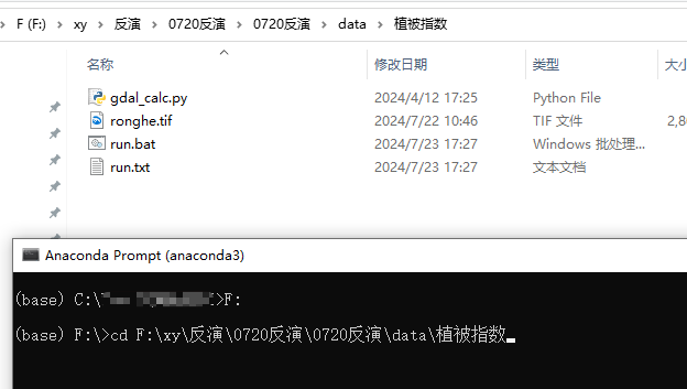
1. 打开Anaconda Prompt。
2. 输入以下命令进入相应的驱动器和目录：

   F:
   cd path\to\your\folder
   

3. 输入并运行批处理文件：

   run.bat
   

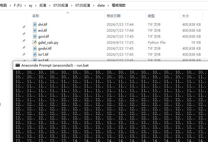
运行后，批处理文件将自动依次执行每个命令，计算所有植被指数，并将结果保存到相应的文件中。

6. 结果展示

每条命令运行后，对应的植被指数会保存在文件夹中，黑窗里的数字到99就代表计算完了一个植被指数。只需等待一小会儿，即可计算完所有的植被指数计算。

7. 总结

通过本文介绍的方法，使用GDAL库可以高效地批量计算植被指数，大大提高了工作效率。批处理文件的使用使得整个过程更加自动化和简便。希望这篇0基础教程能帮助大家更好地掌握GDAL的使用方法。如果有任何问题或需要进一步的帮助，请在评论区留言。
欢迎关注我的公众号：python与遥感，或许里面有你想要的免费教程。