监督学习 | 决策树之网络搜索

相关文章：

机器学习 | 目录

监督学习 | ID3 决策树原理及Python实现

监督学习 | ID3 & C4.5 决策树原理

监督学习 | CART 分类回归树原理

监督学习 | 决策树之Sklearn实现

监督学习 | 决策树之网络搜索

1. 通过网格搜索完善模型

在本文中，我们将为决策树模型拟合一些样本数据。 这个初始模型会过拟合。 然后，我们将使用网格搜索为这个模型找到更好的参数，以减少过拟合。

首先，导入所需要的库：

%matplotlib inline
import pandas as pd
import numpy as np
import matplotlib.pyplot as plt

1.1 数据导入

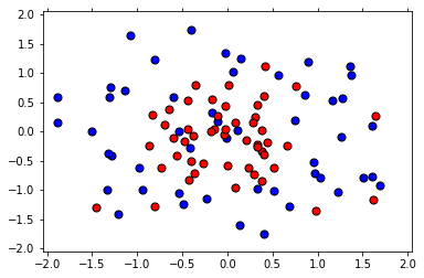
首先定义一个函数用于读取 csv 数据并进行可视化：

def load_pts(csv_name):
    data = np.asarray(pd.read_csv(csv_name, header=None))
    X = data[:,0:2]
    y = data[:,2]

    plt.scatter(X[np.argwhere(y==0).flatten(),0], X[np.argwhere(y==0).flatten(),1],s = 50, color = 'blue', edgecolor = 'k')
    plt.scatter(X[np.argwhere(y==1).flatten(),0], X[np.argwhere(y==1).flatten(),1],s = 50, color = 'red', edgecolor = 'k')
    
    plt.xlim(-2.05,2.05)
    plt.ylim(-2.05,2.05)
    plt.grid(False)
    plt.tick_params(
        axis='x',
        which='both',
        bottom='off',
        top='off')

    return X,y

X, y = load_pts('Data/data.csv')
plt.show()

1.2 拆分数据为训练集和测试集

from sklearn.model_selection import train_test_split
from sklearn.metrics import f1_score, make_scorer

#Fixing a random seed
import random
random.seed(42)

# Split the data into training and testing sets
X_train, X_test, y_train, y_test = train_test_split(X, y, test_size=0.2, random_state=42)

1.3 拟合决策树模型

from sklearn.tree import DecisionTreeClassifier

# Define the model (with default hyperparameters)
clf = DecisionTreeClassifier(random_state=42)

# Fit the model
clf.fit(X_train, y_train)

# Make predictions
train_predictions = clf.predict(X_train)
test_predictions = clf.predict(X_test)

现在我们来可视化模型，并测试 f1_score，首先定义可视化函数：

def plot_model(X, y, clf):
    
    # 绘制两类点的散点图
    plt.scatter(X[np.argwhere(y==0).flatten(),0],X[np.argwhere(y==0).flatten(),1],s = 50, color = 'blue', edgecolor = 'k')
    plt.scatter(X[np.argwhere(y==1).flatten(),0],X[np.argwhere(y==1).flatten(),1],s = 50, color = 'red', edgecolor = 'k')

    # 图形设置
    plt.xlim(-2.05,2.05)
    plt.ylim(-2.05,2.05)
    plt.grid(False)
    plt.tick_params(
        axis='x',
        which='both',
        bottom='off',
        top='off')

    # 利用 np.meshgrid(r,r) 生成一个平面对于的横纵坐标
    r = np.linspace(-2.1,2.1,300)
    s,t = np.meshgrid(r,r)
    
    # 将坐标转换为与决策树的训练集相同格式
    s = np.reshape(s,(np.size(s),1))
    t = np.reshape(t,(np.size(t),1))
    h = np.concatenate((s,t),1)

    # 对平面上的每一个点进行预测类别
    z = clf.predict(h)

    # 将横纵坐标及对应类别转换为矩阵形式
    s = s.reshape((np.size(r),np.size(r)))
    t = t.reshape((np.size(r),np.size(r)))
    z = z.reshape((np.size(r),np.size(r)))

    # 利用 plt.contourf 绘制不同等高面
    plt.contourf(s,t,z,colors = ['blue','red'],alpha = 0.2,levels = range(-1,2))
    
    # 绘制等高面边缘
    if len(np.unique(z)) > 1:
        plt.contour(s,t,z,colors = 'k', linewidths = 2)
    plt.show()

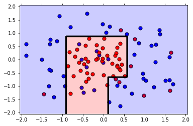
plot_model(X, y, clf)
print('The Training F1 Score is', f1_score(train_predictions, y_train))
print('The Testing F1 Score is', f1_score(test_predictions, y_test))

The Training F1 Score is 1.0
The Testing F1 Score is 0.7000000000000001

训练集得分为 1 ，而测试集得分为 0.7，可以看出当前模型有些过拟合，下面我们通过网络搜索来优化参数。

1.4 使用网络搜索完善模型

现在，我们将执行以下步骤：

1.首先，定义一些参数来执行网格搜索：max_depth, min_samples_leaf, 和 min_samples_split。

2.使用f1_score，为模型制作记分器。

3.使用参数和记分器，在分类器上执行网格搜索。

4.将数据拟合到新的分类器中。

5.绘制模型并找到 f1_score。

6.如果模型不太好，则更改参数的范围并再次拟合。

from sklearn.metrics import make_scorer
from sklearn.model_selection import GridSearchCV

clf = DecisionTreeClassifier(random_state=42)

# 生成参数列表
parameters = {'max_depth':[2,4,6,8,10],'min_samples_leaf':[2,4,6,8,10], 'min_samples_split':[2,4,6,8,10]}

# 定义计分器
scorer = make_scorer(f1_score)

# 生成网络搜索器
grid_obj = GridSearchCV(clf, parameters, scoring=scorer)

# 拟合网络搜索器
grid_fit = grid_obj.fit(X_train, y_train)

# 获得最佳决策树模型
best_clf = grid_fit.best_estimator_

# 对最佳模型进行拟合
best_clf.fit(X_train, y_train)

# 对测试集和训练集进行预测
best_train_predictions = best_clf.predict(X_train)
best_test_predictions = best_clf.predict(X_test)

# 计算测试集得分和训练集得分
print('The training F1 Score is', f1_score(best_train_predictions, y_train))
print('The testing F1 Score is', f1_score(best_test_predictions, y_test))

# 模型可视化
plot_model(X, y, best_clf)

# 查看最佳模型的参数设置
best_clf

The training F1 Score is 0.8148148148148148
The testing F1 Score is 0.8

DecisionTreeClassifier(class_weight=None, criterion='gini', max_depth=4,
                       max_features=None, max_leaf_nodes=None,
                       min_impurity_decrease=0.0, min_impurity_split=None,
                       min_samples_leaf=2, min_samples_split=2,
                       min_weight_fraction_leaf=0.0, presort=False,
                       random_state=42, splitter='best')

由此可以看出，最佳参数为：

max_depth=4

min_samples_leaf=2

min_samples_split=2

且相对于第一个图，边界更为简单，这意味着它不太可能过拟合。

1.5 交叉验证可视化

首先看一下不同参数下的信息：

results = pd.DataFrame(grid_obj.cv_results_)
results.T

	0	1	2	3	4	5	6	7	8	9	...	115	116	117	118	119	120	121	122	123	124
mean_fit_time	0.000536919	0.000609636	0.00067091	0.0005006	0.000532627	0.000538429	0.00162276	0.000725031	0.000346661	0.000960668	...	0.000691652	0.000363668	0.00054733	0.000414769	0.000365416	0.000314713	0.000483354	0.000389099	0.000378688	0.000585318
std_fit_time	7.36079e-05	0.000217965	0.000120917	7.64067e-05	0.000118579	0.000201879	0.00125017	0.000257437	2.95338e-05	0.000841452	...	0.00027542	3.20732e-05	0.000166427	5.31612e-05	2.22742e-05	5.03509e-06	0.000156771	0.000113168	6.09452e-05	0.000168713
mean_score_time	0.00124542	0.00209157	0.0011754	0.00118478	0.00127451	0.00132982	0.00173569	0.00158167	0.000804345	0.00165256	...	0.00107495	0.000776132	0.0010496	0.00107972	0.000799974	0.000889381	0.00097998	0.000957966	0.00082167	0.00108504
std_score_time	0.000460223	0.00131765	0.000217313	0.000175357	0.000274129	0.000684221	0.00012585	0.000531796	2.83336e-05	0.00103978	...	0.000327278	1.61637e-05	0.000181963	0.000226213	3.18651e-05	0.00015253	0.000282182	0.00014771	5.40954e-05	0.00015636
param_max_depth	2	2	2	2	2	2	2	2	2	2	...	10	10	10	10	10	10	10	10	10	10
param_min_samples_leaf	2	2	2	2	2	4	4	4	4	4	...	8	8	8	8	8	10	10	10	10	10
param_min_samples_split	2	4	6	8	10	2	4	6	8	10	...	2	4	6	8	10	2	4	6	8	10
params	{'max_depth': 2, 'min_samples_leaf': 2, 'min_s...	{'max_depth': 2, 'min_samples_leaf': 2, 'min_s...	{'max_depth': 2, 'min_samples_leaf': 2, 'min_s...	{'max_depth': 2, 'min_samples_leaf': 2, 'min_s...	{'max_depth': 2, 'min_samples_leaf': 2, 'min_s...	{'max_depth': 2, 'min_samples_leaf': 4, 'min_s...	{'max_depth': 2, 'min_samples_leaf': 4, 'min_s...	{'max_depth': 2, 'min_samples_leaf': 4, 'min_s...	{'max_depth': 2, 'min_samples_leaf': 4, 'min_s...	{'max_depth': 2, 'min_samples_leaf': 4, 'min_s...	...	{'max_depth': 10, 'min_samples_leaf': 8, 'min_...	{'max_depth': 10, 'min_samples_leaf': 8, 'min_...	{'max_depth': 10, 'min_samples_leaf': 8, 'min_...	{'max_depth': 10, 'min_samples_leaf': 8, 'min_...	{'max_depth': 10, 'min_samples_leaf': 8, 'min_...	{'max_depth': 10, 'min_samples_leaf': 10, 'min...	{'max_depth': 10, 'min_samples_leaf': 10, 'min...	{'max_depth': 10, 'min_samples_leaf': 10, 'min...	{'max_depth': 10, 'min_samples_leaf': 10, 'min...	{'max_depth': 10, 'min_samples_leaf': 10, 'min...
split0_test_score	0.642857	0.642857	0.642857	0.642857	0.642857	0.642857	0.642857	0.642857	0.642857	0.642857	...	0.642857	0.642857	0.642857	0.642857	0.642857	0.642857	0.642857	0.642857	0.642857	0.642857
split1_test_score	0.764706	0.764706	0.764706	0.764706	0.764706	0.764706	0.764706	0.764706	0.764706	0.764706	...	0.5	0.5	0.5	0.5	0.5	0.5	0.5	0.5	0.5	0.5
split2_test_score	0.709677	0.709677	0.709677	0.709677	0.709677	0.709677	0.709677	0.709677	0.709677	0.709677	...	0.714286	0.714286	0.714286	0.714286	0.714286	0.666667	0.666667	0.666667	0.666667	0.666667
mean_test_score	0.705698	0.705698	0.705698	0.705698	0.705698	0.705698	0.705698	0.705698	0.705698	0.705698	...	0.617857	0.617857	0.617857	0.617857	0.617857	0.602381	0.602381	0.602381	0.602381	0.602381
std_test_score	0.0501306	0.0501306	0.0501306	0.0501306	0.0501306	0.0501306	0.0501306	0.0501306	0.0501306	0.0501306	...	0.0889995	0.0889995	0.0889995	0.0889995	0.0889995	0.0737135	0.0737135	0.0737135	0.0737135	0.0737135
rank_test_score	14	14	14	14	14	14	14	14	14	14	...	42	42	42	42	42	62	62	62	62	62

14 rows × 125 columns

接着我们来看一下在不同的最大深度（max_depth）下，每片叶子的最小样本数（min_samples_leaf）和每次分裂的最小样本数（min_samples_split）对决策树模型的泛化性能的影响。

首先定义一个函数来绘制不同最大深度下的热力图（需安装 mglearn）：

def hotmap(max_depth, results):
    fliter = results[results['param_max_depth']==max_depth]
    scores = np.array(fliter['mean_test_score']).reshape(5, 5)
    mglearn.tools.heatmap(scores, xlabel='min_samples_split', xticklabels=parameters['min_samples_split'],
                      ylabel='min_samples_leaf', yticklabels=parameters['min_samples_leaf'], cmap="viridis")

绘制到子图中：

import matplotlib.pyplot as plt 
plt.figure(figsize=(20, 20))
plt
for i in [1,2,3,4,5]:
    plt.subplot(1,5,i, title='max_depth={}'.format(2*i))
    hotmap(2*i, results)

从图中可以看出，每次分裂的最小样本数（min_samples_split）对模型几乎没有影响，而随着最大深度（max_depth）的增加，模型得分逐渐降低。

1.5 总结

通过使用网格搜索，我们将 F1 分数从 0.7 提高到 0.8（同时我们失去了一些训练分数，但这没问题）。 另外，如果你看绘制的图，第二个模型的边界更为简单，这意味着它不太可能过拟合。