A brief presentation about PINN

什么是PINN

要回答什么时PINN，首先要回答什么是PDE，即我们的研究对象，

PDE

关于$u(t,x,y)$的偏微分方程(PDE)，形如
$$f\left(\mathbf{x};\frac{\partial u}{\partial x_1},\dots ,\frac{\partial u}{\partial x_d};\frac{{\partial }^{2}u}{\partial x_1\partial x_1},\dots ,\frac{{\partial }^{2}u}{\partial x_1\partial x_d}\right)=0,\mathbf{x}\in \Omega$$
该等式称为PDE constraints，其中$f(\cdot )$是自变量$\mathbf{x}=\left(x_1,\dots ,x_d\right)$，未知函数u以及u的有限多个偏导数的已知函数，

• 通常会有边值条件:：给定u在空间边界上的取值((Boundary Value Condition, BC)
  $$\mathcal{B}(u,\mathbf{x})=0\text{ on }\partial \Omega$$

• 初值条件((Initial Value Condition, IC)：给定某些自变量值函数初值，例如
  $$u(0,x_2,x_3)=u_0(x_2,x_3)$$
  也可以含有高阶微分的更复杂的形式

• 受数据驱动的观点影响, 有时候会遇到一些具体的数据观测集
  D = { ( x i , u i ) } D=\left\{\left(\mathbf{x}_{i}, u_{i}\right)\right\} D={(xi​,ui​)}
  使得方程满足
  $$u\left({\mathbf{x}}_i\right)=u_i,\forall {\mathbf{x}}_i,u_i\in D$$
  将其称为Data Constraints(DC)

传统方法

传统的基于网格的数值方法例如有限元方法（FEM），有限差分方法（FDM）等，这些方法虽然广泛用于求解PDE，但是却有着一些限制：

• 当维度增加的时候，基于网格的方法会出现维度灾难，无法求解的问题
• 求解只在网格点处计算，非网格点值往往通过差值的方法得到，引入了误差
  而采用神经网络万能逼近的功能去拟合

PINN

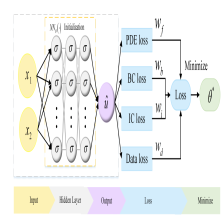
PINN的主要思想，先构建一个输出结果为$\hat{u}$的MLP神经网络，将其作为PDE解的代理模型，将PDE信息作为约束，编码到神经网络损失函数中进行训练。PINN的损失大致可分为PDE loss、BC loss 和 IC loss，在后续研究中又增加了DC loss，表示如下

图1 PINN 示意图

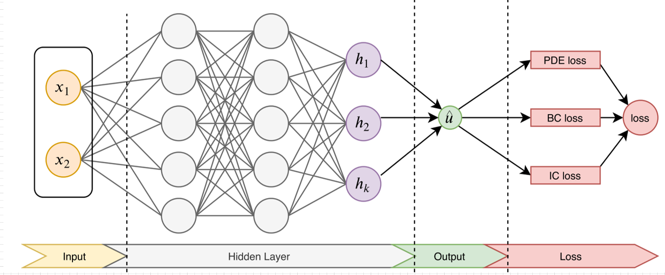
首先构建MLP：

全连接层：
$$\begin{array}{ll}{L}_1(x):=W_{1}x+b_1,& W_1\in {\mathbb{R}}^{d_1\times d},b_1\in {\mathbb{R}}^{d_1}\\ L_k(x):=W_{k}x+b_k,& W_{ik}\in {\mathbb{R}}^{d_k\times d_{k-1}},b_k\in {\mathbb{R}}^{d_k},\forall k=2,3,\cdots D-1\\ L_D(x):=W_{D}x+b_D,& W_D\in {\mathbb{R}}^{N\times d_{D-1}},b_D\in {\mathbb{R}}^N\end{array}$$
再通过激活函数$\sigma$构建如下一个MLP网络
$$N_{\Theta }:=L_D\circ \sigma \circ L_{D-1}\circ \sigma \circ \cdots \circ \sigma \circ L_1$$
第一层W的宽度由输入变量的维数决定最后一层的高度由输出变量的维数决定

将·MLP神经网络作为PDE解的代理模型构建$loss$
$$\mathcal{L}\left(\mathbf{\theta }\right)={\mathcal{L}}_{PDE}\left(\mathbf{\theta };{\mathcal{T}}_f\right)+{\mathcal{L}}_{IC}\left(\mathbf{\theta };{\mathcal{T}}_i\right)+{\mathcal{L}}_{BC}\left(\mathbf{\theta },;{\mathcal{T}}_b\right)+{\mathcal{L}}_{DC}\left(\mathbf{\theta },;{\mathcal{T}}_{data}\right)$$
其中
$$\begin{array}{rl}{\mathcal{L}}_{PDE}\left(\mathbf{\theta };{\mathcal{T}}_f\right)& =\frac{1}{\left|{\mathcal{T}}_f\right|}\sum _{\mathbf{x}\in {\mathcal{T}}_f}{\Vert f\left(\mathbf{x};\frac{\partial \hat{u}}{\partial x_1},\dots ,\frac{\partial \hat{u}}{\partial x_d};\frac{{\partial }^2\hat{u}}{\partial x_1\partial x_1},\dots ,\frac{{\partial }^2\hat{u}}{\partial x_1\partial x_d}\right)\Vert }_2^2\\ {\mathcal{L}}_{IC}\left(\mathbf{\theta };{\mathcal{T}}_i\right)& =\frac{1}{\left|{\mathcal{T}}_i\right|}\sum _{\mathbf{x}\in {\mathcal{T}}_i}\Vert \hat{u}(\mathbf{x})-u(\mathbf{x}){\Vert }_2^2\\ {\mathcal{L}}_{BC}\left(\mathbf{\theta };{\mathcal{T}}_b\right)& =\frac{1}{\left|{\mathcal{T}}_b\right|}\sum _{\mathbf{x}\in {\mathcal{T}}_b}\Vert \mathcal{B}(\hat{u},\mathbf{x}){\Vert }_2^2\\ {\mathcal{L}}_{Data}\left(\mathbf{\theta };{\mathcal{T}}_{data}\right)& =\frac{1}{\left|{\mathcal{T}}_{data}\right|}\sum _{\mathbf{x}\in {\mathcal{T}}_{data}}\Vert \hat{u}(\mathbf{x})-u(\mathbf{x}){\Vert }_2^2\end{array}$$
${\mathcal{T}}_f$，${\mathcal{T}}_i$、${\mathcal{T}}_b$和${\mathcal{T}}_{data}$表示来自PDE，初值、边值以及真值的residual points

最后再通过最小化损失函数$N_{\Theta }$训练

简而言之，所谓的PINN, 就是通过约束和极小化loss的形式训练的神经网络, 满足物理方程及各种定解条件

PINN研究现状

PINN提出

• Dissanayake, MWMG, and N. Phan-Thien. Neural-Network-
  Based Approximations for Solving Partial Differential Equations, 1994. 前面的内容已经被首次提出

• Raissi, M., et al. Physics-Informed Neural Networks: A Deep
  Learning Framework for Solving Forward and Inverse Problems
  Involving Nonlinear Partial Differential Equations. JCP, 2019. 17年
  底, 由布朗大学应用数学系的Raissi等人基于数据驱动的观点将PINN重新提出

• Weinan, E., and Bing Yu. The Deep Ritz Method: A Deep Learning-Based Numerical Algorithm for Solving Variational Problems. Communications in Mathematics and Statistics, 2018, Weinan E 等人也在这个时间点基于变分极小化的观点独立重新提出了PINN
  定义问题，解决工程问题

• Variational Physics-Informed Neural Networks For Solving Partial Differential Equations

• hp-VPINNs: Variational Physics-Informed Neural Networks With Domain Decomposition
  Physics-informed neural networks for inverse problems in nano-optics and metamaterials

• Physics-Informed Neural Networks for Cardiac Activation Mapping

• Non-invasive Inference of Thrombus Material Properties with Physics-informed Neural Networks

• SciANN: A Keras wrapper for scientific computations and physics-informed deep learning using artificial neural networks

网络结构的选择

• Adaptive activation functions accelerate convergence in deep and physics-informed neural networks
• A composite neural network that learns from multi-fidelity data: Application to function approximation and inverse PDE problems
• Weak adversarial networks for high-dimensional partial differential equations

与不确定性结合

• Adversarial Uncertainty Quantification in Physics-Informed Neural Networks
• B-PINNs: Bayesian Physics-Informed Neural Networks for Forward and Inverse PDE Problems with Noisy Data
• Pang G., Karniadakis G.E. (2020) Physics-Informed Learning Machines for Partial Differential Equations: Gaussian Processes Versus Neural Networks. In: Kevrekidis P., Cuevas-Maraver J., Saxena A. (eds) Emerging Frontiers in Nonlinear Science. Nonlinear Systems and Complexity, vol 32. Springer, Cham

loss的选择

• A Dual-Dimer Method for Training Physics-Constrained Neural Networks with Minimax Architecture
• Neural networks catching up with finite differences in solving partial differential equations in higher dimensions
• Multi-Task Learning Using Uncertainty to Weigh Losses for Scene Geometry and Semantics

优化算法

• PPINN: Parareal Physics-Informed Neural Network for time-dependent PDEs（将时间并行的 Parareal 算法用到了 PINN 上）
• A Derivative-Free Method for Solving Elliptic Partial Differential Equations with Deep Neural Networks

PINN加速方法

作为一种数值方法，计算速度同样也是必须的，所以在加速PINN这方面也得到了广泛研究，典型的研究包括
加速训练

• Meng, Xuhui, et al. PPINN: Parareal Physics-Informed Neural Network for Time-Dependent PDEs. ArXiv 2019. 基于时域上的并行, 将PINN应用到传统的parareal算法中, - Dwivedi, Vikas, et al. Distributed Physics Informed Neural Network for Data-Efficient Solution to Partial Differential Equations. , 2019. 尽管神经网络有万能逼近性能, 但逼近一
  个复杂函数的开销也很大, 所以基于空间分解的并行, 将复杂区域分解为诸多小区域, 每个区域由更简单的神经网络来逼近在粗网格时域上用传统数值方法求初始解, 由PINN分别对每个短时域分别训练
• Wang, Sifan, et al. Understanding and Mitigating Gradient Pathologies in Physics-Informed Neural Networks. ArXiv 2020. 之前提到了多种loss, 训练中多个loss的权重也会影响训练速度, 提出了基于梯度大小的加权算法来调整权重

调节网络结构：

• Weinan, E., and Bing Yu. The Deep Ritz Method: A Deep Learning-Based Numerical Algorithm for Solving Variational Problems, 2018. Weinan E在他们重新发现PINN的文章中, 利用了深度学习中的残差网络, 来构造逼近函数, 通常来讲, 残差网络允许构建的层数更深, 有
  更强的表达能力
• Berg, Jens, and Kaj Nyström. A Unified Deep Artificial Neural Network Approach to Partial Differential Equations in Complex Geometrie. Neurocomputing, 2018. PINN的一大优势是无网格, 对于复杂几何区域, 这篇文章进一步利用这一优点, 将PINN分解为三个子网络分别学习边界/到边界的距离/其他物理信息, 进而可以处理较复杂的几何区域
• Peng, Wei, Weien Zhou, Jun Zhang, and Wen Yao. Accelerating Physics-Informed Neural Network Training with Prior Dictionaries
• A. D. Jagtap, K. Kawaguchi, G. E. Karniadakis, Adaptive activation functions accelerate convergence in deep and physics-informed neural networks, Journal of Computational Physics 404 (2020) 109136.