Fourier Features Let Networks Learn High Frequency Functions in Low Dimensional Domains论文笔记

论文信息

题目：
Fourier Features Let Networks Learn High Frequency Functions in Low Dimensional Domains

作者及单位：
Matthew Tancik1∗ Pratul P. Srinivasan1;2∗ Ben Mildenhall1∗ Sara Fridovich-Keil1 Nithin Raghavan1 Utkarsh Singhal1 Ravi Ramamoorthi3 Jonathan T. Barron2 Ren Ng1
1University of California, Berkeley
2Google Research
3University of California, San Diego

期刊、会议：
Computer Vision and Pattern Recognition

时间：18

论文地址：论文链接

代码：

基础

摘要

我们证明通过一个简单的傅里叶特征映射传递输入点可以使多层感知器(MLP)学习低维问题域中的高频函数。因为使用来自神经切线核( the neural tangent kernel, NTK)文献的工具，我们表明一个标准的MLP在理论和实践中都不能学习高频。为了克服这种光谱偏差，我们使用傅里叶特征映射将有效的NTK转换为具有可调带宽的平稳核。我们提出了一种选择特定问题的傅里叶特征的方法，可以极大地提高MLPs在与计算机视觉和图形领域相关的低维回归任务中的性能

论文动机

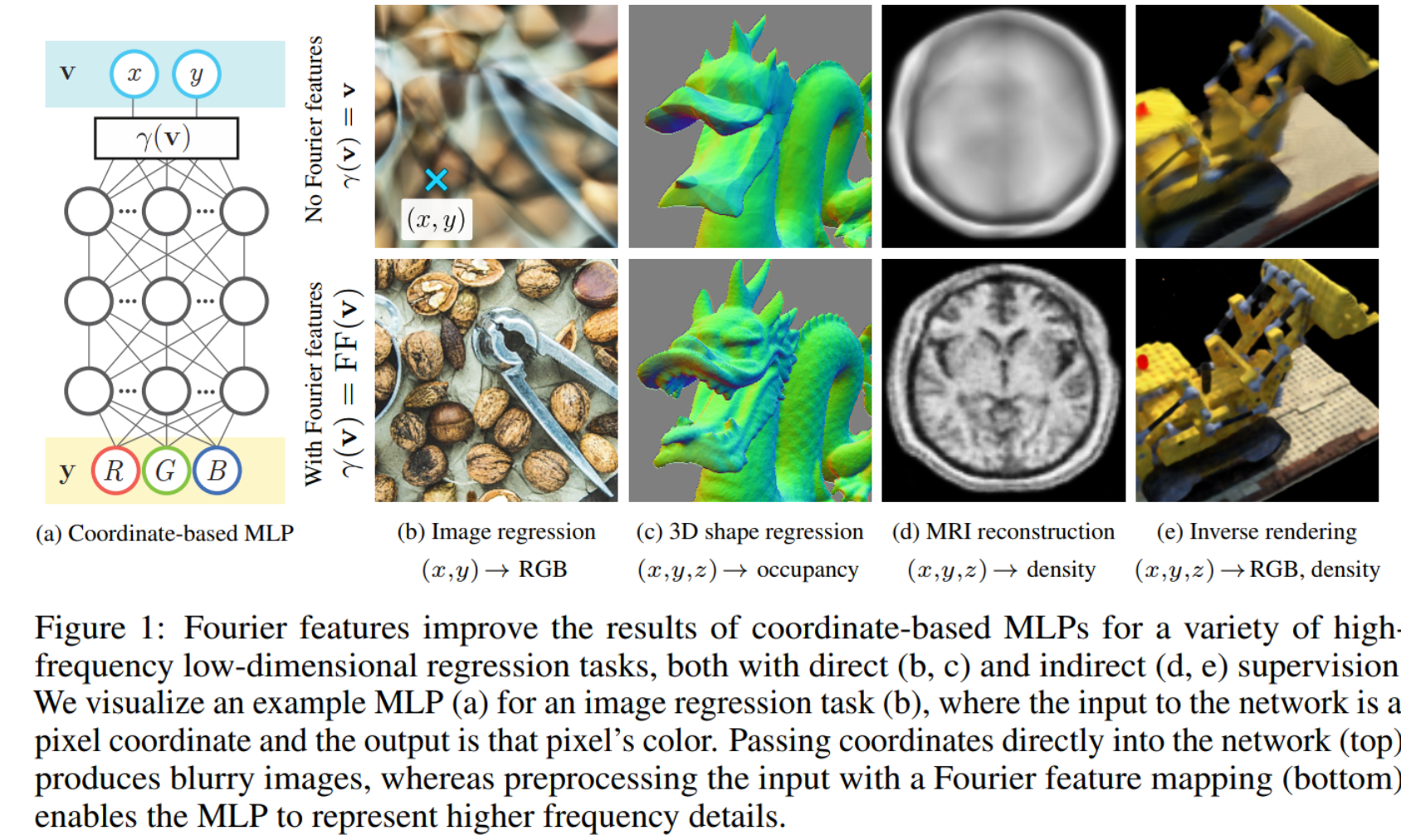
• “基于坐标的”MLPs，以低维坐标作为输入(通常是$R^3$中的点)，并被训练输出每个输入位置的形状、密度和/或颜色的表示. 这个策略是引人注目的，因为基于坐标的MLPs能够适应基于梯度的优化和机器学习，并且可以比网格采样表示更紧凑.
  
• 利用最近在深度网络行为建模方面的进展，使用核回归与神经切核(NTK)[16]从理论上和实验上表明，标准MLPs不适合这些低维的基于坐标的视觉和图形任务。MLPs在学习高频函数方面有困难，在文献中称为“光谱偏差”[3,33]。NTK理论认为，这是因为基于标准坐标的MLPs对应的内核频率衰减较快，这有效地阻止了它们能够代表自然图像和场景中出现的高频内容。即标准MLPs在表示高频内容上有困难
• 最近的一些研究[27,44]通过实验发现，输入坐标的一种启发式正弦映射(称为“位置编码”)允许MLPs表示更高频率的内容
• 考虑一个特别的例子，在输入到MLP前将$\gamma$做这样的映射，$\gamma (\mathbf{v})={\left[a_1\cos \left(2\pi {\mathbf{b}}_1^{\mathrm{T}}\mathbf{v}\right),a_1\sin \left(2\pi {\mathbf{b}}_1^{\mathrm{T}}\mathbf{v}\right),\dots ,a_m\cos \left(2\pi {\mathbf{b}}_m^{\mathrm{T}}\mathbf{v}\right),a_m\sin \left(2\pi {\mathbf{b}}_m^{\mathrm{T}}\mathbf{v}\right)\right]}^{\mathrm{T}}$，然后发现这样的映射使得NTK转化为一个更稳定核，通过修正频率矢量$b_j$能调整NTK的频谱，因而能够控制频率范围，从而能被MLP很好的学习，如图1所示，采用了傅里叶特征的方法MLP学的更好.

Main contributions:

• 我们利用NTK理论和简单的实验表明，傅里叶特征映射可以用来克服基于坐标的MLPs对低频的光谱偏差，允许它们学习更高的频率.
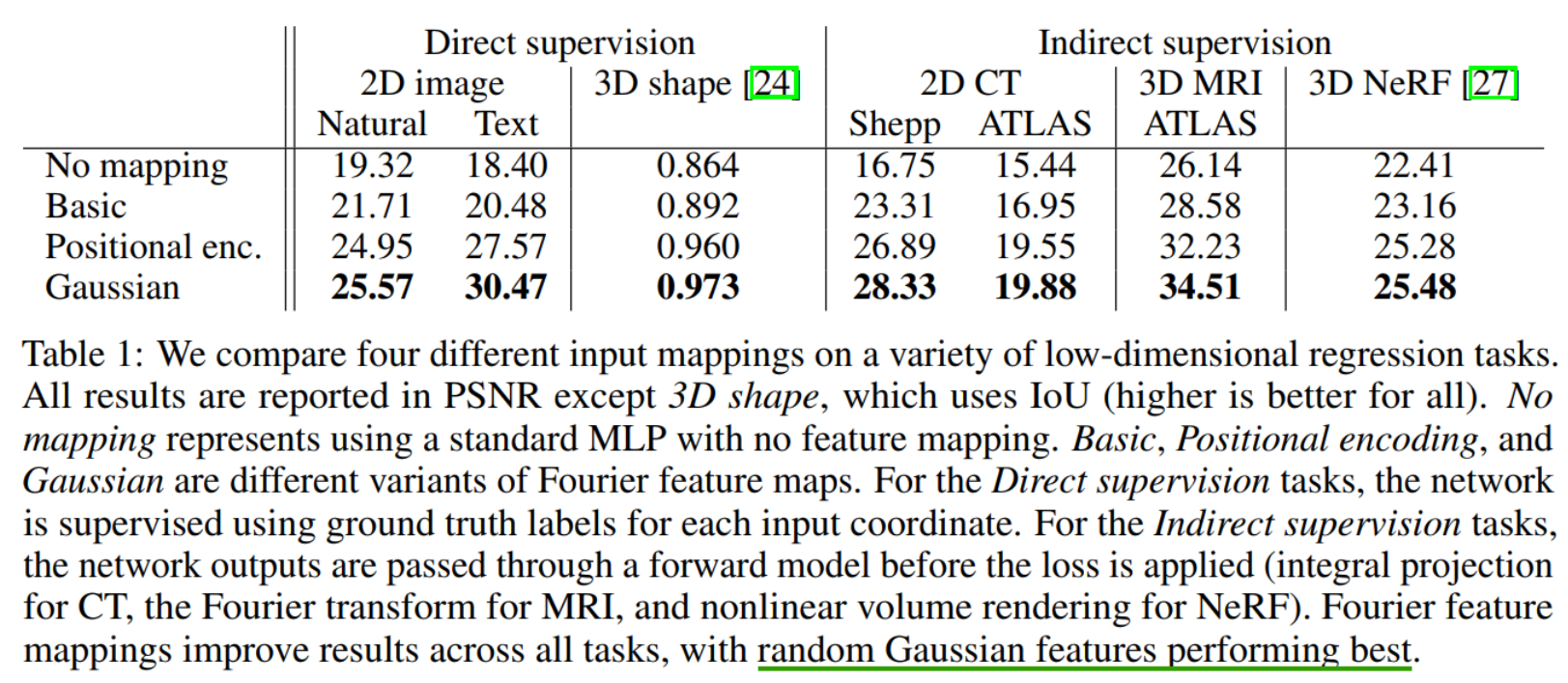
• 我们证明了一个随机的傅里叶特征映射与适当选择的尺度可以显著地提高基于坐标的MLPs在计算机视觉和图形学中许多低维任务的性能.

Related Work

之前在自然语言处理和时间序列分析方面的工作[18,39,42]使用了类似的位置编码来表示时间或一维位置。特别是，Xu等人[42]使用随机傅里叶特征(RFF)[34]来近似使用正弦输入映射的平稳核，并提出了调整映射参数的技术。我们的工作通过直接解释来扩展这一点映射作为最终网络的NTK的修改。此外，我们解决了多维坐标的嵌入，这是必要的视觉和图形任务。

问题背景与定义

• Kernel regression
  a training dataset: ( X , y ) = { ( x i , y i ) } i = 1 n (\mathbf{X}, \mathbf{y})=\left\{\left(\mathbf{x}_{i}, y_{i}\right)\right\}_{i=1}^{n} (X,y)={(xi​,yi​)}i=1n​,其中$x_i$是输入点，$y_i$是对应输出label，核回归是构建一个对任何点x的潜在函数的估计值$\hat{f}$
  $$\hat{f}(\mathbf{x})=\sum _{i=1}^n{\left({\mathbf{K}}^{-1}\mathbf{y}\right)}_{i}k\left({\mathbf{x}}_i,\mathbf{x}\right)$$
  其中，K是$n\times n$核矩阵，${\mathbf{K}}_{ij}=k\left({\mathbf{x}}_i,{\mathbf{x}}_j\right)$，k是对称正半正定核(PSD)函数，代表两个输入矢量的"Similarity"
• Approximating deep networks with kernel regression
  Let $f$ be a fully-connected deep networkwith weights $\theta$ initialized from a Gaussian distribution $N$. The function $f(\mathbf{x};\theta )$ converges over the course of training to the kernel regression solution using the neural tangent kernel (NTK), defined as:
  $$k_{\mathrm{N}\mathrm{T}\mathrm{K}}\left({\mathbf{x}}_i,{\mathbf{x}}_j\right)={\mathbb{E}}_{\theta \sim \mathcal{N}}⟨\frac{\partial f\left({\mathbf{x}}_i;\theta \right)}{\partial \theta },\frac{\partial f\left({\mathbf{x}}_j;\theta \right)}{\partial \theta }⟩$$
  The network’s output for any data Xtest after t training iterations can be approximated as:
  ${\hat{\mathbf{y}}}^{(t)}\approx {\mathbf{K}}_{\mathrm{t}\mathrm{e}\mathrm{s}\mathrm{t}}{\mathbf{K}}^{-1}\left(\mathbf{I}-e^{-\eta \mathbf{K}t}\right)\mathbf{y}$
  其中，${\hat{\mathbf{y}}}^{(t)}=f\left({\mathbf{X}}_{\text{test }};\theta \right)$是在训练迭代t次下对输入${\mathbf{X}}_{\text{test }}$预测
• Spectral bias when training neural networks
  ${\mathbf{Q}}^{\mathrm{T}}\left({\hat{\mathbf{y}}}_{\mathrm{t}\mathrm{r}\mathrm{a}\mathrm{i}\mathrm{n}}^{(t)}-\mathbf{y}\right)\approx {\mathbf{Q}}^{\mathrm{T}}\left(\left(\mathbf{I}-e^{-\eta \mathbf{K}t}\right)\mathbf{y}-\mathbf{y}\right)=-e^{-\eta \mathbf{\Lambda }t}{\mathbf{Q}}^{\mathrm{T}}\mathbf{y}$

本文方法

Fourier Features for a Tunable Stationary Neural Tangent Kernel
$\gamma (\mathbf{v})={\left[a_1\cos \left(2\pi {\mathbf{b}}_1^{\mathrm{T}}\mathbf{v}\right),a_1\sin \left(2\pi {\mathbf{b}}_1^{\mathrm{T}}\mathbf{v}\right),\dots ,a_m\cos \left(2\pi {\mathbf{b}}_m^{\mathrm{T}}\mathbf{v}\right),a_m\sin \left(2\pi {\mathbf{b}}_m^{\mathrm{T}}\mathbf{v}\right)\right]}^{\mathrm{T}}$
由于$\cos (\alpha -\beta )=\cos \alpha \cos \beta +\sin \alpha \sin \beta$，The kernel function induced by this mapping is
$$k_{\gamma }\left({\mathbf{v}}_1,{\mathbf{v}}_2\right)=\gamma {\left({\mathbf{v}}_1\right)}^{\mathrm{T}}\gamma \left({\mathbf{v}}_2\right)=\sum _{j=1}^m{a}_j^2\cos \left(2\pi {\mathbf{b}}_j^{\mathrm{T}}\left({\mathbf{v}}_1-{\mathbf{v}}_2\right)\right)=h_{\gamma }\left({\mathbf{v}}_1-{\mathbf{v}}_2\right)$$
其中
$$h_{\gamma }\left({\mathbf{v}}_{\Delta }\right)\triangleq \sum _{j=1}^m{a}_j^2\cos \left(2\pi {\mathbf{b}}_j^{\mathrm{T}}{\mathbf{v}}_{\Delta }\right)$$
Note that this kernel is stationary (a function of only the difference between points). We can think of the mapping as a Fourier approximation of a kernel function， ${\mathbf{b}}_j$ are the Fourier basis frequencies used to approximate the kernel. $a_j^2$ are the corresponding Fourier series coefficients.

In our case, ${\mathbf{x}}_i=\gamma \left({\mathbf{v}}_i\right)$ so the composed kernel becomes
$h_{\mathrm{N}\mathrm{T}\mathrm{K}}\left({\mathbf{x}}_i^{\mathrm{T}}{\mathbf{x}}_j\right)=h_{\mathrm{N}\mathrm{T}\mathrm{K}}\left(\gamma {\left({\mathbf{v}}_i\right)}^{\mathrm{T}}\gamma \left({\mathbf{v}}_j\right)\right)=h_{\mathrm{N}\mathrm{T}\mathrm{K}}\left(h_{\gamma }\left({\mathbf{v}}_i-{\mathbf{v}}_j\right)\right)$
因此，在这些嵌入的输入点上训练一个网络就相当于使用平稳的组成NTK函数进行核回归$h_{\mathrm{N}\mathrm{T}\mathrm{K}}\circ h_{\gamma }$. MLP函数在每个输入训练点${\mathbf{v}}_i$ 用一个加权的Dirac函数近似地对组成的NTK进行卷积
$\hat{f}=\left(h_{\mathrm{N}\mathrm{T}\mathrm{K}}\circ h_{\gamma }\right)\ast {\sum }_{i=1}^n{w}_i{\delta }_{{\mathbf{v}}_i}$
$\mathbf{w}={\mathbf{K}}^{-1}\mathbf{y}$

Relevant literature

数值实验

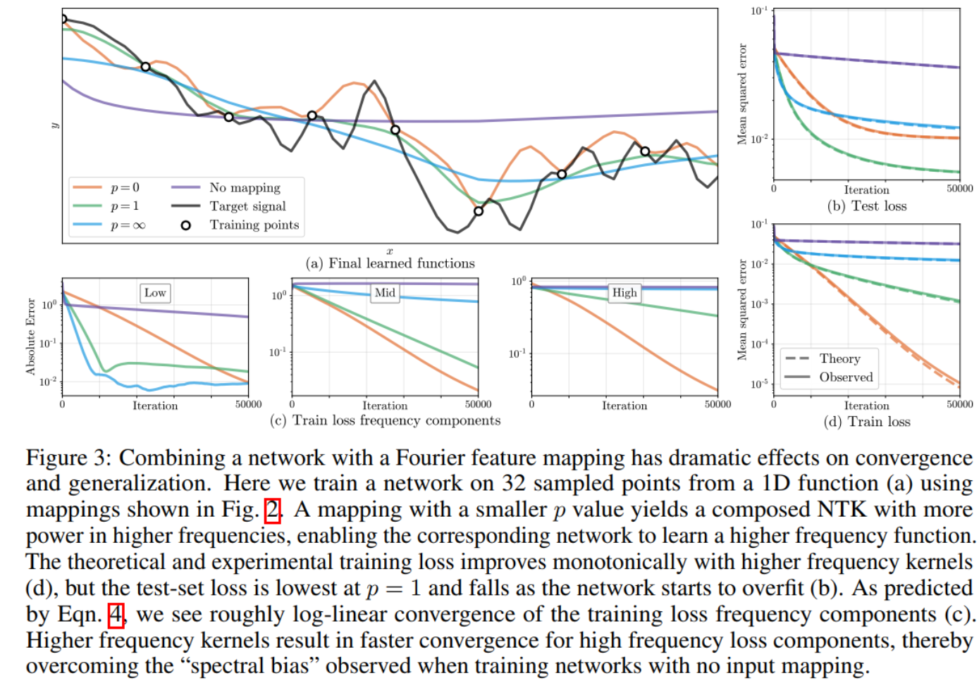
In Figure 3, we train MLPs (4 layers, 1024 channels, ReLU activations) to fit a bandlimited $1/f^1$ noise signal (c = 8; n = 32) using Fourier feature mappings with different p values. Figures 3b and 3d show that the NTK linear dynamics model accurately predict the effects of modifying the Fourier feature mapping parameters. Separating different frequency components of the training error in Figure 3c reveals that networks with narrower NTK spectra converge faster for low frequency components but essentially never converge for high frequency components, whereas networks with wider NTK spectra successfully converge across all components. The Fourier feature mapping p = 1 has adequate power across frequencies present in the target signal (so the network converges rapidly during training) but limited power in higher frequencies (preventing overfitting or aliasing).

Neural Network Approximation Theorem for PDEs

总结：

我们利用NTK理论来证明傅里叶特征映射可以使基于坐标的MLPs更适合低维的建模功能，从而克服基于坐标的MLPs固有的光谱偏差。我们的实验表明，调整傅里叶特征参数提供了对组合NTK频率衰减的控制，并显著提高了一系列图形和成像任务的性能。，这些发现阐明了在计算机视觉和图形管道中使用基于协调的MLPs来表示3D形状的新兴技术，并为从业者提供了一个简单的策略来改善这些领域的结果