蓝桥云 NumPy 百题大冲关

基础部分

1.导入 NumPy：
import numpy as np
2. 查看 NumPy 版本信息：
np.version

创建数组

NumPy 的主要对象是多维数组 Ndarray。在 NumPy 中维度 Dimensions 叫做轴 Axes，轴的个数叫做秩 Rank。注意，numpy.array 和 Python 标准库 array.array 并不相同，前者更为强大，这也就是我们学习 NumPy 的重要原因之一。
3. 通过列表创建一维数组：
np.array([1, 2, 3])
上方数组是一个秩为 1 的数组，因为它只有一个轴，而轴的长度为 3。
4. 通过列表创建二维数组：
np.array([(1, 2, 3), (4, 5, 6)])
上方数组的秩为 2。第一个维度长度为 2,第二个维度长度为 3。
5. 创建全为 0 的二维数组：
np.zeros((3,3))
array([[0., 0., 0.],
[0., 0., 0.],
[0., 0., 0.]])

6.创建全为 1 的三维数组：
np.ones((2,3,4))
array([[[1., 1., 1., 1.],
[1., 1., 1., 1.],
[1., 1., 1., 1.]],
[[1., 1., 1., 1.],
[1., 1., 1., 1.],
[1., 1., 1., 1.]]])

7.创建一维等差数组：
np.arange(5)
array([0, 1, 2, 3, 4])
8. 创建二维等差数组：
np.arange(6).reshape(2, 3)
array([[0, 1, 2],
[3, 4, 5]])
9. 创建单位矩阵（二维数组）：
np.eye(3)
array([[1., 0., 0.],
[0., 1., 0.],
[0., 0., 1.]])
10. 创建等间隔一维数组：
np.linspace(1, 10, num=6)
array([ 1. , 2.8, 4.6, 6.4, 8.2, 10. ])
11. 创建二维随机数组：
np.random.rand(2, 3)
12. 创建二维随机整数数组（数值小于 5）：
np.random.randint(5, size=(2, 3))
13. 依据自定义函数创建数组：
np.fromfunction(lambda i, j: i + j, (3, 3))

数组运算

生成一维示例数组：
a = np.array([10, 20, 30, 40, 50])
b = np.arange(1, 6)
a, b

14.一维数组加法运算：
15. 一维数组减法运算：
16. 一维数组乘法运算：
17. 一维数组除法运算：

生成二维示例数组（可以看作矩阵）：
18.矩阵加法运算：
A + B
19. 矩阵减法运算：
A - B
20. 矩阵元素间乘法运算：
A * B
np.dot(A, B)
21. 矩阵乘法运算（注意与上题的区别）：
np.dot(A, B)
如果使用 np.mat 将二维数组准确定义为矩阵，就可以直接使用 * 完成矩阵乘法计算。
np.mat(A) * np.mat(B)
22.数乘矩阵：
2 * A
23. 矩阵的转置：
A.T
24. 矩阵求逆：
np.linalg.inv(A)

数学函数

25.三角函数：
print(a)
np.sin(a)
[10 20 30 40 50]
array([-0.54402111, 0.91294525, -0.98803162, 0.74511316, -0.26237485])
26. 以自然对数函数为底数的指数函数：
np.exp(a)
27.数组的方根的运算（开平方）：
np.sqrt(a)
28.数组的方根的运算（立方）：
np.power(a, 3)

数组切片和索引

29.一维数组索引：
a = np.array([1, 2, 3, 4, 5])
a[0], a[-1]
(1, 5)
30. 一维数组切片：
a[0:2], a[:-1]
(array([1, 2]), array([1, 2, 3, 4]))
31.二维数组索引
a = np.array([(1, 2, 3), (4, 5, 6), (7, 8, 9)])
a[0], a[-1]
(array([1, 2, 3]), array([7, 8, 9]))
32.二维数组切片（取第2列）
print(a)
a[:, 1]
[[1 2 3]
[4 5 6]
[7 8 9]]
array([2, 5, 8])
33.二维数组切片（取第2，3行）
a[1:3, :]
array([[4, 5, 6],
[7, 8, 9]])

数组形状操作

a = np.random.random((3, 2))
a
array([[0.10574785, 0.89013732],
[0.67778593, 0.239752 ],
[0.35651587, 0.4972274 ]])

34.查看数组形状：
a.shape
(3, 2)
35.更改数组形状（不改变原始数组）：
a.reshape(2, 3)
array([[0.10574785, 0.89013732, 0.67778593],
[0.239752 , 0.35651587, 0.4972274 ]])

a
array([[0.10574785, 0.89013732],
[0.67778593, 0.239752 ],
[0.35651587, 0.4972274 ]])

36.更改数组形状（改变原始数组）
a.resize(2, 3)
a
array([[0.10574785, 0.89013732, 0.67778593],
[0.239752 , 0.35651587, 0.4972274 ]])

37.展平数组
a.ravel()
array([0.10574785, 0.89013732, 0.67778593, 0.239752 , 0.35651587,
0.4972274 ])
38.垂直拼合数组
a = np.random.randint(10, size=(3, 3))
b = np.random.randint(10, size=(3, 3))
a, b
(array([[4, 9, 8],
[9, 4, 4],
[6, 8, 2]]), array([[0, 4, 2],
[3, 1, 0],
[4, 9, 7]]))
np.vstack((a, b))
array([[4, 9, 8],
[9, 4, 4],
[6, 8, 2],
[0, 4, 2],
[3, 1, 0],
[4, 9, 7]])
39.水平拼合数组
np.hstack((a, b))
array([[4, 9, 8, 0, 4, 2],
[9, 4, 4, 3, 1, 0],
[6, 8, 2, 4, 9, 7]])
40.沿横轴分割数组
np.hsplit(a, 3)
[array([[4],
[9],
[6]]), array([[9],
[4],
[8]]), array([[8],
[4],
[2]])]
41.沿纵轴分割数组
np.vsplit(a, 3)
[array([[4, 9, 8]]), array([[9, 4, 4]]), array([[6, 8, 2]])]

数组排序

a = np.array(([1, 4, 3], [6, 2, 9], [4, 7, 2]))
a
array([[1, 4, 3],
[6, 2, 9],
[4, 7, 2]])

42.返回每列最大值
np.max(a, axis=0)
array([6, 7, 9])
43.返回每行最小值
np.min(a, axis=1)
array([1, 2, 2])
44.返回每列最大值索引
np.argmax(a, axis=0)
array([1, 2, 1])
45.返回每行最小值索引
np.argmin(a, axis=1)
array([0, 1, 2])

数组统计

46.统计数组各列的中位数：
np.median(a, axis=0)
47.统计数组各行的算术平均值：
np.mean(a, axis=1)
48.统计数组各列的加权平均值：
np.average(a, axis=0)
49.统计数组各行的方差：
np.var(a, axis=1)
50.统计数组各列的标准偏差：
np.std(a, axis=0)

进阶部分

51.创建一个 5x5 的二维数组，其中边界值为1，其余值为0：
Z = np.ones((5, 5))
Z[1:-1, 1:-1] = 0
Z

array([[1., 1., 1., 1., 1.],
[1., 0., 0., 0., 1.],
[1., 0., 0., 0., 1.],
[1., 0., 0., 0., 1.],
[1., 1., 1., 1., 1.]])
52.使用数字 0 将一个全为 1 的 5x5 二维数组包围
Z = np.ones((5, 5))
Z = np.pad(Z, pad_width=1, mode=‘constant’, constant_values=0)
Z

array([[0., 0., 0., 0., 0., 0., 0.],
[0., 1., 1., 1., 1., 1., 0.],
[0., 1., 1., 1., 1., 1., 0.],
[0., 1., 1., 1., 1., 1., 0.],
[0., 1., 1., 1., 1., 1., 0.],
[0., 1., 1., 1., 1., 1., 0.],
[0., 0., 0., 0., 0., 0., 0.]])

53.创建一个 5x5 的二维数组，并设置值 1, 2, 3, 4 落在其对角线下方：
Z = np.diag(1+np.arange(4), k=-1)
Z
array([[0, 0, 0, 0, 0],
[1, 0, 0, 0, 0],
[0, 2, 0, 0, 0],
[0, 0, 3, 0, 0],
[0, 0, 0, 4, 0]])

54.创建一个 10x10 的二维数组，并使得 1 和 0 沿对角线间隔放置：
Z = np.zeros((10, 10), dtype=int)
Z[1::2, ::2] = 1
Z[::2, 1::2] = 1
Z
array([[0, 1, 0, 1, 0, 1, 0, 1, 0, 1],
[1, 0, 1, 0, 1, 0, 1, 0, 1, 0],
[0, 1, 0, 1, 0, 1, 0, 1, 0, 1],
[1, 0, 1, 0, 1, 0, 1, 0, 1, 0],
[0, 1, 0, 1, 0, 1, 0, 1, 0, 1],
[1, 0, 1, 0, 1, 0, 1, 0, 1, 0],
[0, 1, 0, 1, 0, 1, 0, 1, 0, 1],
[1, 0, 1, 0, 1, 0, 1, 0, 1, 0],
[0, 1, 0, 1, 0, 1, 0, 1, 0, 1],
[1, 0, 1, 0, 1, 0, 1, 0, 1, 0]])

55.创建一个 0-10 的一维数组，并将 (1, 9] 之间的数全部反转成负数：
Z = np.arange(11)
Z[(1 < Z) & (Z <= 9)] *= -1
Z

array([ 0, 1, -2, -3, -4, -5, -6, -7, -8, -9, 10])

56.找出两个一维数组中相同的元素：
Z1 = np.random.randint(0, 10, 10)
Z2 = np.random.randint(0, 10, 10)
print(“Z1:”, Z1)
print(“Z2:”, Z2)
np.intersect1d(Z1, Z2)

Z1: [5 0 4 0 3 7 8 3 4 1]
Z2: [7 6 5 6 2 2 3 3 2 7]
array([3, 5, 7])

57.使用 NumPy 打印昨天、今天、明天的日期：
yesterday = np.datetime64(‘today’, ‘D’) - np.timedelta64(1, ‘D’)
today = np.datetime64(‘today’, ‘D’)
tomorrow = np.datetime64(‘today’, ‘D’) + np.timedelta64(1, ‘D’)
print("yesterday: ", yesterday)
print("today: ", today)
print("tomorrow: ", tomorrow)

yesterday: 2019-11-11
today: 2019-11-12
tomorrow: 2019-11-13

58.使用五种不同的方法去提取一个随机数组的整数部分：
Z = np.random.uniform(0, 10, 10)
print("原始值: ", Z)

print("方法 1: ", Z - Z % 1)
print("方法 2: ", np.floor(Z))
print("方法 3: ", np.ceil(Z)-1)
print("方法 4: ", Z.astype(int))
print("方法 5: ", np.trunc(Z))

原始值: [6.00778092 5.80556614 7.15667395 5.93362201 9.22395203 8.07950897
5.47478339 5.73771434 1.1287305 8.4555598 ]
方法 1: [6. 5. 7. 5. 9. 8. 5. 5. 1. 8.]
方法 2: [6. 5. 7. 5. 9. 8. 5. 5. 1. 8.]
方法 3: [6. 5. 7. 5. 9. 8. 5. 5. 1. 8.]
方法 4: [6 5 7 5 9 8 5 5 1 8]
方法 5: [6. 5. 7. 5. 9. 8. 5. 5. 1. 8.]

59.创建一个 5x5 的矩阵，其中每行的数值范围从 1 到 5：
Z = np.zeros((5, 5))
Z += np.arange(1, 6)

Z
array([[1., 2., 3., 4., 5.],
[1., 2., 3., 4., 5.],
[1., 2., 3., 4., 5.],
[1., 2., 3., 4., 5.],
[1., 2., 3., 4., 5.]])

60.创建一个长度为 5 的等间隔一维数组，其值域范围从 0 到 1，但是不包括 0 和 1：
Z = np.linspace(0, 1, 6, endpoint=False)[1:]

Z
array([0.16666667, 0.33333333, 0.5 , 0.66666667, 0.83333333])

61.创建一个长度为10的随机一维数组，并将其按升序排序：
Z = np.random.random(10)
Z.sort()
Z
array([0.0952028 , 0.1889449 , 0.2909388 , 0.36923433, 0.45031452,
0.5232143 , 0.67872147, 0.7910516 , 0.81933846, 0.97431475])

62.创建一个 3x3 的二维数组，并将列按升序排序：
Z = np.array([[7, 4, 3], [3, 1, 2], [4, 2, 6]])
print(“原始数组: \n”, Z)

Z.sort(axis=0)
Z

原始数组:
[[7 4 3]
[3 1 2]
[4 2 6]]

array([[3, 1, 2],
[4, 2, 3],
[7, 4, 6]])

63.创建一个长度为 5 的一维数组，并将其中最大值替换成 0：
Z = np.random.random(5)
print("原数组: ", Z)
Z[Z.argmax()] = 0
Z

原数组: [0.97383452 0.52031187 0.08380792 0.16240293 0.56919927]

array([0. , 0.52031187, 0.08380792, 0.16240293, 0.56919927])

64.打印每个 NumPy 标量类型的最小值和最大值：
for dtype in [np.int8, np.int32, np.int64]:
print("The minimum value of {}: ".format(dtype), np.iinfo(dtype).min)
print("The maximum value of {}: ".format(dtype), np.iinfo(dtype).max)
for dtype in [np.float32, np.float64]:
print("The minimum value of {}: ".format(dtype), np.finfo(dtype).min)
print("The maximum value of {}: ".format(dtype), np.finfo(dtype).max)

The minimum value of <class ‘numpy.int8’>: -128
The maximum value of <class ‘numpy.int8’>: 127
The minimum value of <class ‘numpy.int32’>: -2147483648
The maximum value of <class ‘numpy.int32’>: 2147483647
The minimum value of <class ‘numpy.int64’>: -9223372036854775808
The maximum value of <class ‘numpy.int64’>: 9223372036854775807
The minimum value of <class ‘numpy.float32’>: -3.4028235e+38
The maximum value of <class ‘numpy.float32’>: 3.4028235e+38
The minimum value of <class ‘numpy.float64’>: -1.7976931348623157e+308
The maximum value of <class ‘numpy.float64’>: 1.7976931348623157e+308

65.将 float32 转换为整型：
Z = np.arange(10, dtype=np.float32)
print(Z)

Z = Z.astype(np.int32, copy=False)
Z

[0. 1. 2. 3. 4. 5. 6. 7. 8. 9.]
array([0, 1, 2, 3, 4, 5, 6, 7, 8, 9], dtype=int32)

66.将随机二维数组按照第 3 列从上到下进行升序排列：
Z = np.random.randint(0, 10, (5, 5))
print(“排序前：\n”, Z)

Z[Z[:, 2].argsort()]

排序前：
[[2 3 3 8 2]
[2 4 3 8 6]
[8 0 0 2 5]
[2 5 4 7 8]
[6 6 5 9 9]]

array([[8, 0, 0, 2, 5],
[2, 3, 3, 8, 2],
[2, 4, 3, 8, 6],
[2, 5, 4, 7, 8],
[6, 6, 5, 9, 9]])

67.从随机一维数组中找出距离给定数值（0.5）最近的数：
Z = np.random.uniform(0, 1, 20)
print(“随机数组: \n”, Z)
z = 0.5
m = Z.flat[np.abs(Z - z).argmin()]

m

随机数组:
[0.83469649 0.60623978 0.36243098 0.69344754 0.66498498 0.15069018
0.3722634 0.83249527 0.89010024 0.32616245 0.81209585 0.98237687
0.11632099 0.16045724 0.54638975 0.26279212 0.93678775 0.06922646
0.22921632 0.99611394]

0.5463897464314816

68.将二维数组的前两行进行顺序交换：
A = np.arange(25).reshape(5, 5)
print(A)
A[[0, 1]] = A[[1, 0]]
print(A)

[[ 0 1 2 3 4]
[ 5 6 7 8 9]
[10 11 12 13 14]
[15 16 17 18 19]
[20 21 22 23 24]]
[[ 5 6 7 8 9]
[ 0 1 2 3 4]
[10 11 12 13 14]
[15 16 17 18 19]
[20 21 22 23 24]]

69.找出随机一维数组中出现频率最高的值：
Z = np.random.randint(0, 10, 50)
print(“随机一维数组:”, Z)
np.bincount(Z).argmax()

随机一维数组: [0 8 7 1 2 6 2 2 8 7 9 7 5 9 7 3 9 7 6 5 7 4 4 9 1 5 5 6 1 1 9 9 6 9 1 1 5
2 6 5 6 4 8 6 2 2 1 5 6 1]

1

70.找出给定一维数组中非 0 元素的位置索引：
Z = np.nonzero([1, 0, 2, 0, 1, 0, 4, 0])
Z
(array([0, 2, 4, 6]),)

71.对于给定的 5x5 二维数组，在其内部随机放置 p 个值为 1 的数：
p = 3

Z = np.zeros((5, 5))
np.put(Z, np.random.choice(range(5*5), p, replace=False), 1)

Z

array([[0., 0., 0., 0., 1.],
[0., 1., 0., 0., 0.],
[0., 0., 0., 0., 0.],
[0., 0., 0., 0., 0.],
[0., 1., 0., 0., 0.]])

72.对于随机的 3x3 二维数组，减去数组每一行的平均值：
X = np.random.rand(3, 3)
print(X)

Y = X - X.mean(axis=1, keepdims=True)
Y

[[0.94481763 0.71885257 0.64564054]
[0.26427321 0.44115571 0.80828852]
[0.6223677 0.94623723 0.14231897]]

array([[ 0.17504738, -0.05091768, -0.12412971],
[-0.24029927, -0.06341677, 0.30371604],
[ 0.05205973, 0.37592927, -0.427989 ]])

73.获得二维数组点积结果的对角线数组：
A = np.random.uniform(0, 1, (3, 3))
B = np.random.uniform(0, 1, (3, 3))

print(np.dot(A, B))

较慢的方法
np.diag(np.dot(A, B))

[[0.80406101 1.07890552 0.8916094 ]
[0.09906674 0.34654188 0.19145505]
[0.68164007 1.11179246 0.82322019]]

array([0.80406101, 0.34654188, 0.82322019])

74.找到随机一维数组中前 p 个最大值：
Z = np.random.randint(1, 100, 100)
print(Z)

p = 5

Z[np.argsort(Z)[-p:]]

[48 7 4 30 50 14 71 58 14 23 58 54 99 36 22 53 14 56 83 14 23 74 8 82
32 98 48 40 42 52 70 42 97 24 98 52 66 53 98 86 82 36 43 58 74 40 65 75
6 31 89 22 35 18 85 62 24 52 6 66 92 70 28 20 7 76 58 19 29 61 93 54
94 31 53 49 65 11 67 7 3 61 52 49 57 21 42 85 6 97 69 19 94 2 6 96
75 89 2 34]

array([97, 98, 98, 98, 99])

75.计算随机一维数组中每个元素的 4 次方数值：
x = np.random.randint(2, 5, 5)
print(x)

np.power(x, 4)

76.对于二维随机数组中各元素，保留其 2 位小数：
Z = np.random.random((5, 5))
print(Z)

np.set_printoptions(precision=2)
Z

[[0.00617658 0.34882944 0.79642325 0.89031641 0.23249308]
[0.9148618 0.18720168 0.95517613 0.92058836 0.21316617]
[0.56028522 0.24435398 0.519926 0.89318027 0.60469563]
[0.66392006 0.5480811 0.69831084 0.24848752 0.86348583]
[0.79082676 0.74613623 0.78593804 0.6535201 0.46029704]]

array([[0.01, 0.35, 0.8 , 0.89, 0.23],
[0.91, 0.19, 0.96, 0.92, 0.21],
[0.56, 0.24, 0.52, 0.89, 0.6 ],
[0.66, 0.55, 0.7 , 0.25, 0.86],
[0.79, 0.75, 0.79, 0.65, 0.46]])

77.使用科学记数法输出 NumPy 数组：
Z = np.random.random([5, 5])
print(Z)

Z/1e3

[[0.28 0.59 0.08 0.4 0.04]
[0.65 0.49 0.81 0.66 0.16]
[0.47 0.8 0.89 0.71 0.1 ]
[0.48 0.19 0.48 0.4 0.8 ]
[0.99 0.4 0.16 0.08 0.58]]

array([[2.78e-04, 5.92e-04, 7.82e-05, 4.01e-04, 4.31e-05],
[6.51e-04, 4.87e-04, 8.07e-04, 6.60e-04, 1.58e-04],
[4.70e-04, 8.05e-04, 8.94e-04, 7.07e-04, 1.05e-04],
[4.78e-04, 1.91e-04, 4.81e-04, 4.05e-04, 7.95e-04],
[9.86e-04, 3.98e-04, 1.56e-04, 7.90e-05, 5.81e-04]])

78.使用 NumPy 找出百分位数（25%，50%，75%）：
a = np.arange(15)
print(a)

np.percentile(a, q=[25, 50, 75])

[ 0 1 2 3 4 5 6 7 8 9 10 11 12 13 14]

array([ 3.5, 7. , 10.5])
79.找出数组中缺失值的总数及所在位置：
生成含缺失值的 2 维数组
Z = np.random.rand(10, 10)
Z[np.random.randint(10, size=5), np.random.randint(10, size=5)] = np.nan
Z

array([[0.74, 0.1 , 0.43, 0.26, 0.92, 0.07, 0.62, 0.39, 0.42, 0. ],
[0.05, 0.94, 0.66, 0.63, 0.27, 0.87, 0.31, 0.25, 0.68, 0.74],
[0.45, 0.53, 0.99, 0.13, 0.79, 0.96, nan, 0.3 , 0.57, 0.41],
[0.9 , 0.8 , 0.85, 0.16, 0.47, 0.48, 0.63, 0.42, 0.44, 0.67],
[0.56, 0.08, 0.69, 0.8 , 0.55, nan, 0.25, 0.4 , 0.39, 0.39],
[0.28, 0.49, 0.23, 0.67, 0.83, 0.88, 0.48, 0.05, 0.44, 0.66],
[0.7 , 0.71, 0.69, 0.35, 0.58, 0.2 , nan, 0.43, 0.76, 0.89],
[0.94, 0.08, 0.85, 0.61, 0.09, 0.68, 0.51, 0.94, 0.99, 0.96],
[0.62, 0.43, 0.94, 0.23, 0.16, 0.09, 0.57, 0.54, nan, 0.65],
[0.98, 0.83, 0.61, 0.44, 0.46, 0.82, 0.56, 0.46, 0.68, 0.36]])

print(“缺失值总数: \n”, np.isnan(Z).sum())
print(“缺失值索引: \n”, np.where(np.isnan(Z)))

缺失值总数:
4
缺失值索引:
(array([2, 4, 6, 8]), array([6, 5, 6, 8]))

80.从随机数组中删除包含缺失值的行：
沿用 79 题中的含缺失值的 2 维数组
Z[np.sum(np.isnan(Z), axis=1) == 0]
array([[0.74, 0.1 , 0.43, 0.26, 0.92, 0.07, 0.62, 0.39, 0.42, 0. ],
[0.05, 0.94, 0.66, 0.63, 0.27, 0.87, 0.31, 0.25, 0.68, 0.74],
[0.9 , 0.8 , 0.85, 0.16, 0.47, 0.48, 0.63, 0.42, 0.44, 0.67],
[0.28, 0.49, 0.23, 0.67, 0.83, 0.88, 0.48, 0.05, 0.44, 0.66],
[0.94, 0.08, 0.85, 0.61, 0.09, 0.68, 0.51, 0.94, 0.99, 0.96],
[0.98, 0.83, 0.61, 0.44, 0.46, 0.82, 0.56, 0.46, 0.68, 0.36]])

81.统计随机数组中的各元素的数量：
Z = np.random.randint(0, 100, 25).reshape(5, 5)
print(Z)
np.unique(Z, return_counts=True) # 返回值中，第 2 个数组对应第 1 个数组元素的数量

[[11 56 72 90 64]
[64 11 96 81 49]
[82 3 74 86 86]
[83 74 34 43 78]
[25 77 36 69 80]]

(array([ 3, 11, 25, 34, 36, 43, 49, 56, 64, 69, 72, 74, 77, 78, 80, 81, 82,
83, 86, 90, 96]),
array([1, 2, 1, 1, 1, 1, 1, 1, 2, 1, 1, 2, 1, 1, 1, 1, 1, 1, 2, 1, 1]))

82.将数组中各元素按指定分类转换为文本值：
指定类别如下
1 → 汽车
2 → 公交车
3 → 火车

Z = np.random.randint(1, 4, 10)
print(Z)

label_map = {1: “汽车”, 2: “公交车”, 3: “火车”}

[label_map[x] for x in Z]
[1 2 1 1 1 3 3 3 2 3]
[‘汽车’, ‘公交车’, ‘汽车’, ‘汽车’, ‘汽车’, ‘火车’, ‘火车’, ‘火车’, ‘公交车’, ‘火车’]

83.将多个 1 维数组拼合为单个 Ndarray：
Z1 = np.arange(3)
Z2 = np.arange(3, 7)
Z3 = np.arange(7, 10)

Z = np.array([Z1, Z2, Z3])
print(Z)

np.concatenate(Z)
[array([0, 1, 2]) array([3, 4, 5, 6]) array([7, 8, 9])]
array([0, 1, 2, 3, 4, 5, 6, 7, 8, 9])

84.打印各元素在数组中升序排列的索引：
a = np.random.randint(100, size=10)
print('Array: ', a)
a.argsort()

Array: [ 4 23 57 73 11 95 57 93 19 38]
array([0, 4, 8, 1, 9, 2, 6, 3, 7, 5])

85.得到二维随机数组各行的最大值：
Z = np.random.randint(1, 100, [5, 5])
print(Z)

np.amax(Z, axis=1)

[[91 79 32 23 30]
[15 55 65 43 83]
[96 56 82 2 28]
[47 17 12 18 33]
[89 73 18 20 13]]

array([91, 83, 96, 47, 89])
86.得到二维随机数组各行的最小值（区别上面的方法）：
Z = np.random.randint(1, 100, [5, 5])
print(Z)

np.apply_along_axis(np.min, arr=Z, axis=1)

[[45 95 31 53 60]
[87 97 36 79 32]
[63 91 37 70 25]
[64 25 7 42 88]
[53 44 68 18 40]]

array([31, 32, 25, 7, 18])
87.计算两个数组之间的欧氏距离：
a = np.array([1, 2])
b = np.array([7, 8])

数学计算方法
print(np.sqrt(np.power((8-2), 2) + np.power((7-1), 2)))
NumPy 计算
np.linalg.norm(b-a)
88.打印复数的实部和虚部：
a = np.array([1 + 2j, 3 + 4j, 5 + 6j])

print(“实部：”, a.real)
print(“虚部：”, a.imag)
实部： [1. 3. 5.]
虚部： [2. 4. 6.]
89.求解给出矩阵的逆矩阵并验证：
matrix = np.array([[1., 2.], [3., 4.]])
inverse_matrix = np.linalg.inv(matrix)

验证原矩阵和逆矩阵的点积是否为单位矩阵
assert np.allclose(np.dot(matrix, inverse_matrix), np.eye(2))
inverse_matrix

90.使用 Z-Score 标准化算法对数据进行标准化处理：

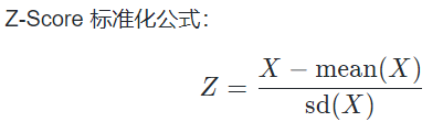
根据公式定义函数
def zscore(x, axis=None):
xmean = x.mean(axis=axis, keepdims=True)
xstd = np.std(x, axis=axis, keepdims=True)
zscore = (x-xmean)/xstd
return zscore

生成随机数据
Z = np.random.randint(10, size=(5, 5))
print(Z)

zscore(Z)
91.使用 Min-Max 标准化算法对数据进行标准化处理：

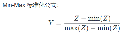
根据公式定义函数
def min_max(x, axis=None):
min = x.min(axis=axis, keepdims=True)
max = x.max(axis=axis, keepdims=True)
result = (x-min)/(max-min)
return result

生成随机数据
Z = np.random.randint(10, size=(5, 5))
print(Z)

min_max(Z)

[[8 5 1 0 4]
[5 0 8 6 0]
[6 2 3 3 7]
[5 1 1 7 5]
[6 8 0 9 4]]

array([[0.89, 0.56, 0.11, 0. , 0.44],
[0.56, 0. , 0.89, 0.67, 0. ],
[0.67, 0.22, 0.33, 0.33, 0.78],
[0.56, 0.11, 0.11, 0.78, 0.56],
[0.67, 0.89, 0. , 1. , 0.44]])
92.使用 L2 范数对数据进行标准化处理：
根据公式定义函数
def l2_normalize(v, axis=-1, order=2):
l2 = np.linalg.norm(v, ord=order, axis=axis, keepdims=True)
l2[l2 == 0] = 1
return v/l2

生成随机数据
Z = np.random.randint(10, size=(5, 5))
print(Z)

l2_normalize(Z)

[[3 1 3 3 6]
[1 3 7 7 4]
[4 6 7 0 1]
[5 8 4 1 6]
[8 3 8 8 0]]

array([[0.38, 0.12, 0.38, 0.38, 0.75],
[0.09, 0.27, 0.63, 0.63, 0.36],
[0.4 , 0.59, 0.69, 0. , 0.1 ],
[0.42, 0.67, 0.34, 0.08, 0.5 ],
[0.56, 0.21, 0.56, 0.56, 0. ]])
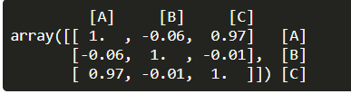
93.使用 NumPy 计算变量直接的相关性系数：
Z = np.array([
[1, 2, 1, 9, 10, 3, 2, 6, 7], # 特征 A
[2, 1, 8, 3, 7, 5, 10, 7, 2], # 特征 B
[2, 1, 1, 8, 9, 4, 3, 5, 7]]) # 特征 C

np.corrcoef(Z)

array([[ 1. , -0.06, 0.97],
[-0.06, 1. , -0.01],
[ 0.97, -0.01, 1. ]])
相关性系数取值从 [-1, 1]变换，靠近 1 则代表正相关性较强，-1则代表负相关性较强。结果如下所示，变量 A 与变量 A 直接的相关性系数为 1，因为是同一个变量。变量 A 与变量 C 之间的相关性系数为 0.97，说明相关性较强。

94.使用 NumPy 计算矩阵的特征值和特征向量：
M = np.matrix([[1, 2, 3], [4, 5, 6], [7, 8, 9]])
w, v = np.linalg.eig(M)
w 对应特征值，v 对应特征向量
w, v
(array([ 1.61e+01, -1.12e+00, -9.76e-16]), matrix([[-0.23, -0.79, 0.41],
[-0.53, -0.09, -0.82],
[-0.82, 0.61, 0.41]]))
我们可以通过 P’AP=M公式反算，验证是否能得到原矩阵。
v * np.diag(w) * np.linalg.inv(v)

95.使用 NumPy 计算 Ndarray 两相邻元素差值：
Z = np.random.randint(1, 10, 10)
print(Z)

计算 Z 两相邻元素差值
print(np.diff(Z, n=1))
重复计算 2 次
print(np.diff(Z, n=2))
重复计算 3 次
print(np.diff(Z, n=3))

[5 2 5 5 3 1 6 8 3 4]
[-3 3 0 -2 -2 5 2 -5 1]
[ 6 -3 -2 0 7 -3 -7 6]
[ -9 1 2 7 -10 -4 13]
96.使用 NumPy 将 Ndarray 相邻元素依次累加：
Z = np.random.randint(1, 10, 10)
print(Z)

“”"
[第一个元素, 第一个元素 + 第二个元素, 第一个元素 + 第二个元素 + 第三个元素, …]
“”"
np.cumsum(Z)
[9 3 5 3 2 2 5 1 7 1]

array([ 9, 12, 17, 20, 22, 24, 29, 30, 37, 38])
97.使用 NumPy 按列连接两个数组：
M1 = np.array([1, 2, 3])
M2 = np.array([4, 5, 6])

np.c_[M1, M2]
array([[1, 4],
[2, 5],
[3, 6]])

98.使用 NumPy 按行连接两个数组：
M1 = np.array([1, 2, 3])
M2 = np.array([4, 5, 6])

np.r_[M1, M2]
array([1, 2, 3, 4, 5, 6])
99.使用 NumPy 打印九九乘法表：
np.fromfunction(lambda i, j: (i + 1) * (j + 1), (9, 9))

100.使用 NumPy 将蓝桥云课 LOGO 转换为 Ndarray 数组：
from io import BytesIO
from PIL import Image
import PIL
import requests
通过链接下载图像
URL = ‘https://static.shiyanlou.com/img/logo-black.png’
response = requests.get(URL)
将内容读取为图像
I = Image.open(BytesIO(response.content))
将图像转换为 Ndarray
shiyanlou = np.asarray(I)
shiyanlou