


自然语言处理笔记总目录
关于人名分类问题:
- 以一个人名为输入,使用模型帮助我们判断它最有可能是来自哪一个国家的人名,这在某些国际化公司的业务中具有重要意义,在用户注册过程中,会根据用户填写的名字直接给他分配可能的国家或地区选项,以及该国家或地区的国旗,限制手机号码位数等等
本案例取自PyTorch官网的NLP FROM SCRATCH: CLASSIFYING NAMES WITH A CHARACTER-LEVEL RNN,在此基础上增加了完整的注释以及通俗的讲解,完整代码在文章最后
本案例没有使用便捷强大的 torchtext 库,可以更深刻的了解到NLP底层的一些工作
实现效果:
$ python predict.py Hinton
(-0.47) Scottish
(-1.52) English
(-3.57) Irish

$ python predict.py Schmidhuber
(-0.19) German
(-2.48) Czech
(-2.68) Dutch
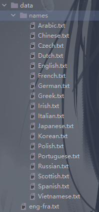
人名分类数据:
本案例大致分为如下步骤
Step 1:Preparing the Data
在本步中,我们将得到一个字典,列出了每种语言的名称列表{language: [names ...]}
from io import open
import glob
import os

def findFiles(path):
    return glob.glob(path)

print(findFiles('data/names/*.txt'))
Out:
['data/names\\Arabic.txt', 'data/names\\Chinese.txt', 'data/names\\Czech.txt',
'data/names\\Dutch.txt', 'data/names\\English.txt', 'data/names\\French.txt',
'data/names\\German.txt', 'data/names\\Greek.txt', 'data/names\\Irish.txt',
'data/names\\Italian.txt', 'data/names\\Japanese.txt', 'data/names\\Korean.txt',
'data/names\\Polish.txt', 'data/names\\Portuguese.txt', 'data/names\\Russian.txt',
'data/names\\Scottish.txt', 'data/names\\Spanish.txt', 'data/names\\Vietnamese.txt']
import unicodedata
import string

# 所有大小写字母以及空格、句号、逗号、分号、引号,共57个
all_letters = string.ascii_letters + " .,;'"
n_letters = len(all_letters) # 57

# 将Unicode字符转换为ASCII
# 简而言之这个函数的作用就是去除某些语音中的重音标记
# 比如:Ślusàrski --> Slusarski
def unicodeToAscii(s):
    return ''.join(
        c for c in unicodedata.normalize('NFD', s)
        if unicodedata.category(c) != 'Mn'
        and c in all_letters
    )

print(unicodeToAscii('Ślusàrski'))
Out:
Slusarski
# 字典category_lines:键为语言,值为保存一个所有名字的列表
# 列表all_categories:保存所有语言名
category_lines = {}
all_categories = []

# 读取文件并进行分割形成列表
def readLines(filename):
    # read()将整个文件读入,strip()去除两侧空白符,使用'\n'进行划分
    lines = open(filename, encoding='utf-8').read().strip().split('\n')
    # 对应每一个lines列表中的名字进行Ascii转换, 使其规范化.最后返回一个名字列表
    return [unicodeToAscii(line) for line in lines]

for filename in findFiles('data/names/*.txt'):
	# findFiles返回了所有文件名
    # basename返回文件名全称,即去除路径
    # splitext将文件名称与后缀分割开,[0]即是取文件名称
    category = os.path.splitext(os.path.basename(filename))[0]
    # 列表all_categories:保存所有语言名
    all_categories.append(category)
    # 字典category_lines:键为语言,值为保存一个所有名字的列表
    lines = readLines(filename)
    category_lines[category] = lines

n_categories = len(all_categories)	# 18
至此,我们拥有了category_lines字典与all_categories语言列表以及n_categories类别总数,供之后的代码使用
# 测试一下
print("all_categories: ", all_categories)
print("Italian: ", category_lines['Italian'][:5])
Out:
all_categories: ['Arabic', 'Chinese', 'Czech', 'Dutch', 'English',
'French', 'German', 'Greek', 'Irish', 'Italian', 'Japanese', 'Korean',
'Polish', 'Portuguese', 'Russian', 'Scottish', 'Spanish', 'Vietnamese']
Italian: ['Abandonato', 'Abatangelo', 'Abatantuono', 'Abate', 'Abategiovanni']
Step 2:Turning Names into Tensors
将名字转换为Tensor,使用什么方法呢?这里为了表示单个字母,我们使用one-hot编码,大小为<1 x n_letters>,即行数为1,列数为总的字符数,上述已经提到,本例中字符总数为57。例如: "b" = <0 1 0 0 0 ...>
为了表示出一个单词张量,这里将维度扩展为<line_length x 1 x n_letters>,第一维是单词的长度,第二维代表批量大小,因为 PyTorch 假定所有内容都是成批的,这里我们使用1代替即可,第三维是总字符数。这个新的维度也可以理解为单词的字母数量 * 每个字母的one-hot编码
import torch

# Find letter index from all_letters, e.g. "a" = 0
def letterToIndex(letter):
    return all_letters.find(letter)

# Just for demonstration, turn a letter into a <1 x n_letters> Tensor
def letterToTensor(letter):
    tensor = torch.zeros(1, n_letters)
    tensor[0][letterToIndex(letter)] = 1
    return tensor

# Turn a line into a <line_length x 1 x n_letters>,
# or an array of one-hot letter vectors
def lineToTensor(line):
    tensor = torch.zeros(len(line), 1, n_letters)
    for li, letter in enumerate(line):
        tensor[li][0][letterToIndex(letter)] = 1
    return tensor

print(letterToTensor('J'))

print(lineToTensor('Jones').size())
Out:
tensor([[0., 0., 0., 0., 0., 0., 0., 0., 0., 0., 0., 0., 0., 0., 0., 0., 0., 0.,
         0., 0., 0., 0., 0., 0., 0., 0., 0., 0., 0., 0., 0., 0., 0., 0., 0., 1.,
         0., 0., 0., 0., 0., 0., 0., 0., 0., 0., 0., 0., 0., 0., 0., 0., 0., 0.,
         0., 0., 0.]])
torch.Size([5, 1, 57])
Step 3:Creating the Network
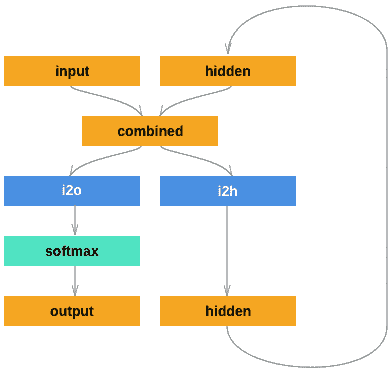
注意:这里的softmax使用的是LogSoftmax
import torch.nn as nn

class RNN(nn.Module):
    def __init__(self, input_size, hidden_size, output_size):
        super(RNN, self).__init__()

        self.hidden_size = hidden_size

        self.i2h = nn.Linear(input_size + hidden_size, hidden_size)
        self.i2o = nn.Linear(input_size + hidden_size, output_size)
        self.softmax = nn.LogSoftmax(dim=1)

    def forward(self, input, hidden):
        combined = torch.cat((input, hidden), 1)
        hidden = self.i2h(combined)
        output = self.i2o(combined)
        output = self.softmax(output)
        return output, hidden

    def initHidden(self):
        return torch.zeros(1, self.hidden_size)

n_hidden = 128
rnn = RNN(n_letters, n_hidden, n_categories)
要使此网络运行,需要传递输入(在本例中为当前字母的张量)和上一步的隐藏状态(首先将其初始化为零)。返回值为输出(每种语言的概率)和下一个隐藏状态(我们将其保留用于下一步)
input = letterToTensor('A')
hidden = torch.zeros(1, n_hidden)

output, next_hidden = rnn(input, hidden)
为了提高效率,而不是每个步骤创建一个新的张量,因此我们将使用lineToTensor而不是letterToTensor并使用切片。 这可以通过预先计算一批张量来进一步优化。
input = lineToTensor('Albert')
hidden = torch.zeros(1, n_hidden)

output, next_hidden = rnn(input[0], hidden)
print(output)
print(output.size())
Out:
tensor([[-2.9245, -2.9573, -2.8859, -2.8642, -2.9882, -2.8798, -2.8757, -2.8279,
         -2.8843, -2.8742, -2.8713, -2.8891, -2.9144, -2.8538, -2.9654, -2.9352,
         -2.7799, -2.8768]], grad_fn=<LogSoftmaxBackward0>)
torch.Size([1, 18])
如上输出,为<1 x n_categories>的张量,每一个数都是该类别的可能性(值越大概率越高)
Step 4:Training
Preparing for Training
在进行训练之前,我们应该构造一些辅助函数。首先就是categoryFromOutput,从网络的输出的张量中得到所属类别以及下标索引
def categoryFromOutput(output):
    # 最大值top_n及其所在下标top_i
    top_n, top_i = output.topk(1)
    category_i = top_i[0].item()
    return all_categories[category_i], category_i

print(categoryFromOutput(output))
Out:
('Portuguese', 13)
我们还将希望有一种快速的方法来获取训练示例(名称及其语言)
import random

def randomChoice(l):
    return l[random.randint(0, len(l) - 1)]

def randomTrainingExample():
	# 首先随机选取一个类别
    category = randomChoice(all_categories)
    # 从随机选取的类别当中随机选取一个名字
    line = randomChoice(category_lines[category])
    # 得到类别张量category_tensor,存放这当前选取类别的下标
    category_tensor = torch.tensor([all_categories.index(category)], dtype=torch.long)
	# 得到名字张量line_tensor,大小为 <line_length x 1 x 57>
    line_tensor = lineToTensor(line)
    return category, line, category_tensor, line_tensor

for i in range(10):
    category, line, category_tensor, line_tensor = randomTrainingExample()
    print('category =', category, '/ line =', line)
Out:
category = Italian / line = Petri
category = Czech / line = Korycan
category = Arabic / line = Asghar
category = Vietnamese / line = Than
category = Polish / line = Wojda
category = Greek / line = Maneates
category = Greek / line = Tselios
category = Scottish / line = Hill
category = Russian / line = Adamovitch
category = Greek / line = Karkampasis
random模块中也有choice方法,也可以直接调用random.choice
Training the Network
现在,我们要向网络中传入大量的示例让它进行预测,并且告诉网络是否预测正确。
对于损失函数,将使用nn.NLLLoss,因为前述提到RNN的最后一层使用的是nn.LogSoftmax,这两个是匹配的,具体原因这里推荐一篇博客【Pytorch详解NLLLoss和CrossEntropyLoss】供参考
criterion = nn.NLLLoss()
Each loop of training will:
- Create input and target tensors
- Create a zeroed initial hidden state
- Read each letter in and
- Keep hidden state for next letter
- Compare final output to target
- Back-propagate
- Return the output and loss
learning_rate = 0.005

def train(category_tensor, line_tensor):
    hidden = rnn.initHidden()

    rnn.zero_grad()

    for i in range(line_tensor.size()[0]):
        output, hidden = rnn(line_tensor[i], hidden)

    loss = criterion(output, category_tensor)
    loss.backward()

    # 更新模型中的参数:optimizer.step()
    for p in rnn.parameters():
        p.data.add_(p.grad.data, alpha=-learning_rate)

    return output, loss.item()
现在,我们只需向网络中喂入大量示例即可。同时,我们可以打印输出以及绘制损失函数图
import time
import math

n_iters = 100000
print_every = 5000
plot_every = 1000


# Keep track of losses for plotting
current_loss = 0
all_losses = []

def timeSince(since):
    now = time.time()
    s = now - since
    m = math.floor(s / 60)
    s -= m * 60
    return '%dm %ds' % (m, s)

start = time.time()

for iter in range(1, n_iters + 1):
    category, line, category_tensor, line_tensor = randomTrainingExample()
    output, loss = train(category_tensor, line_tensor)
    current_loss += loss

    # Print iter number, loss, name and guess
    if iter % print_every == 0:
        guess, guess_i = categoryFromOutput(output)
        correct = '✓' if guess == category else '✗ (%s)' % category
        print('%d %d%% (%s) %.4f %s / %s %s' % (iter, iter / n_iters * 100, timeSince(start), loss, line, guess, correct))

    # Add current loss avg to list of losses
    if iter % plot_every == 0:
        all_losses.append(current_loss / plot_every)
        current_loss = 0
Out:
5000 5% (0m 12s) 2.7593 Guerra / Japanese ✗ (Portuguese)
10000 10% (0m 23s) 3.0733 Bahvaloff / Scottish ✗ (Russian)
15000 15% (0m 34s) 1.7275 Nosek / Czech ✗ (Polish)
20000 20% (0m 44s) 1.6654 Tosi / Italian ✓
25000 25% (0m 54s) 1.2599 Zhilkin / Russian ✓
30000 30% (1m 4s) 2.2486 Deniel / Portuguese ✗ (French)
35000 35% (1m 14s) 0.8166 Tchehluev / Russian ✓
40000 40% (1m 24s) 0.8256 Fei / Chinese ✓
45000 45% (1m 35s) 4.0699 Kool / Korean ✗ (Dutch)
50000 50% (1m 45s) 1.3071 Buckholtz / Scottish ✗ (German)
55000 55% (1m 55s) 0.8277 Vo / Vietnamese ✓
60000 60% (2m 6s) 1.7692 Huang / Vietnamese ✗ (Chinese)
65000 65% (2m 17s) 0.2499 Yim / Korean ✓
70000 70% (2m 29s) 0.0152 Akrivopoulos / Greek ✓
75000 75% (2m 40s) 0.5435 Mooney / Irish ✓
80000 80% (2m 52s) 1.6462 Kieu / Chinese ✗ (Vietnamese)
85000 85% (3m 4s) 4.9142 Samuel / Arabic ✗ (Irish)
90000 90% (3m 15s) 0.3337 Paloumbas / Greek ✓
95000 95% (3m 26s) 0.0426 Kassab / Arabic ✓
100000 100% (3m 37s) 2.6238 Michel / Irish ✗ (Dutch)
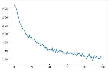
Step 5:Plotting the Results
import matplotlib.pyplot as plt
import matplotlib.ticker as ticker

plt.figure()
plt.plot(all_losses)
Step 6:Evaluating the Results
为了查看网络在不同类别上的表现,我们将创建一个混淆矩阵,行为实际语言,列为网络猜测语言。为了计算混淆矩阵,使用evaluate()通过网络运行一批样本,等同于没有反向传播的train()
# Keep track of correct guesses in a confusion matrix
confusion = torch.zeros(n_categories, n_categories)
n_confusion = 10000

# Just return an output given a line
def evaluate(line_tensor):
    hidden = rnn.initHidden()

    for i in range(line_tensor.size()[0]):
        output, hidden = rnn(line_tensor[i], hidden)

    return output

# Go through a bunch of examples and record which are correctly guessed
for i in range(n_confusion):
    category, line, category_tensor, line_tensor = randomTrainingExample()
    output = evaluate(line_tensor)
    # 预测的类别以及下标
    guess, guess_i = categoryFromOutput(output)
    # 真实的类别的下标
    category_i = all_categories.index(category)
    # 在行为真实类别,列的猜测类别的位置加一
    confusion[category_i][guess_i] += 1

# Normalize by dividing every row by its sum
for i in range(n_categories):
    confusion[i] = confusion[i] / confusion[i].sum()

# Set up plot
fig = plt.figure()
ax = fig.add_subplot(111)
cax = ax.matshow(confusion.numpy())
fig.colorbar(cax)

# Set up axes
ax.set_xticklabels([''] + all_categories, rotation=90)
ax.set_yticklabels([''] + all_categories)

# Force label at every tick
ax.xaxis.set_major_locator(ticker.MultipleLocator(1))
ax.yaxis.set_major_locator(ticker.MultipleLocator(1))

# sphinx_gallery_thumbnail_number = 2
plt.show()
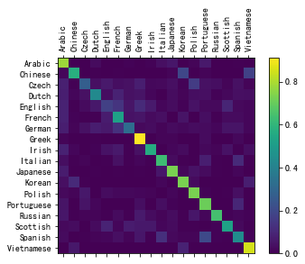
可以稍对此图进行一个分析,比如猜测哪种语言名的性能最好,从图中可以看出Greek相对应的点是最亮的,即次网络对Greek名字的预测性能是最好的。再比如English的猜测是最不准确的,几乎每一个横坐标对应的颜色都是一样的,也就是说喂入网络中一个英文名字,有可能猜测成任意语言而小概率能预测正确。
Step 7:Running on User Input
给定一个名字,输出相对应正确率前三的类别所属
def predict(input_line, n_predictions=3):
    print('\n> %s' % input_line)
    with torch.no_grad():
        output = evaluate(lineToTensor(input_line))

        # Get top N categories
        topv, topi = output.topk(n_predictions, 1, True)
        predictions = []

        for i in range(n_predictions):
            value = topv[0][i].item()
            category_index = topi[0][i].item()
            print('(%.2f) %s' % (value, all_categories[category_index]))
            predictions.append([value, all_categories[category_index]])

predict('Dovesky')
predict('Jackson')
predict('Satoshi')
Out:
> Dovesky
(-0.36) Russian
(-1.75) Czech
(-3.24) English

> Jackson
(-0.80) Scottish
(-1.34) Greek
(-2.34) English

> Satoshi
(-1.10) Italian
(-1.54) Polish
(-1.81) Japanese
最终版本的代码将分为以下几个文件:
data.py(加载文件)model.py(定义 RNN)train.py(进行训练)predict.py(使用命令行参数运行predict())server.py(通过bottle.py将预测用作 JSON API)
运行train.py训练并保存网络
使用名称运行predict.py以查看预测:
$ python predict.py Hazaki
(-0.42) Japanese
(-1.39) Polish
(-3.51) Czech
运行server.py并访问http://localhost:5533/Yourname以获取预测的 JSON 输出。
Exercises
除了上述所用的 nn.RNN 模型,尝试使用 nn.LSTM 和 nn.GRU 层来构建本项目
步骤和上述大致相同,只是更换一下网络的架构以及训练函数,这里就不在放代码了,可以看一下损失函数图
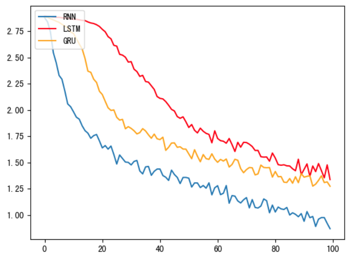
从图中可以看出,LSTM以及GRU的效果都是不如RNN的,原因就是我们现在的文本数据是人名,长度步长并且各个字母之前并无特定关联,因此无法发挥LSTM以及GRU的长距离捕捉语义信息关联的优势,在我们的实际任务当中,我们要通过对任务的分析以及实验的对比,选择出最适合的模型。


 743
743


 被折叠的 条评论
为什么被折叠?
被折叠的 条评论
为什么被折叠?
 到【灌水乐园】发言


