scikit-opt的使用

scikit-opt的使用

一个封装了7种启发式算法的 Python 代码库
（差分进化算法、遗传算法、粒子群算法、模拟退火算法、蚁群算法、鱼群算法、免疫优化算法）

0.安装

pip install scikit-opt

或者直接把源代码中的 sko 文件夹下载下来放本地也调用可以

---

1.差分进化算法(DE)

(Differential Evolution Algorithm，DE)

参数说明

入参	默认值	意义
func	-	目标函数
n_dim	-	目标函数的维度
size_pop	50	种群规模
max_iter	200	最大迭代次数
prob_mut	0.001	变异概率
F	0.5	变异系数
lb	-1	每个自变量的最小值
ub	1	每个自变量的最大值
constraint_eq	空元组	等式约束
constraint_ueq	空元组	不等式约束(<=0)

'''
min f(x1, x2, x3) = x1^2 + x2^2 + x3^2
s.t.
    x1*x2 >= 1
    x1*x2 <= 5
    x2 + x3 = 1
    0 <= x1, x2, x3 <= 5
'''


def obj_func(p):
    x1, x2, x3 = p
    return x1 ** 2 + x2 ** 2 + x3 ** 2


constraint_eq = [
    lambda x: 1 - x[1] - x[2]
]

constraint_ueq = [
    lambda x: 1 - x[0] * x[1],
    lambda x: x[0] * x[1] - 5
]

# %% Do DifferentialEvolution
from sko.DE import DE

de = DE(func=obj_func, n_dim=3, size_pop=50, max_iter=800, lb=[0, 0, 0], ub=[5, 5, 5],
        constraint_eq=constraint_eq, constraint_ueq=constraint_ueq)

best_x, best_y = de.run()
print('best_x:', best_x, '\n', 'best_y:', best_y)

结果

best_x: [1.02276678 0.9785311  0.02146889] 
 best_y: [2.00403592]

---

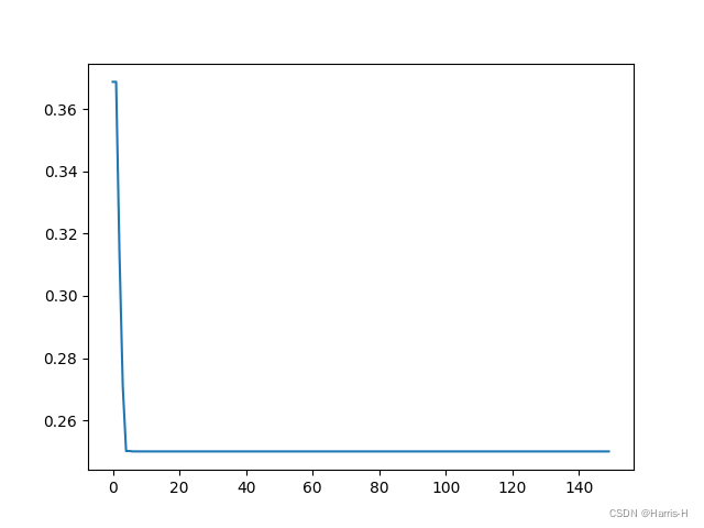
2.粒子群算法(PSO)

def demo_func(x):
    x1, x2, x3 = x
    return x1 ** 2 + (x2 - 0.05) ** 2 + x3 ** 2


# %% Do PSO
from sko.PSO import PSO

pso = PSO(func=demo_func, n_dim=3, pop=40, max_iter=150, lb=[0, -1, 0.5], ub=[1, 1, 1], w=0.8, c1=0.5, c2=0.5)
pso.run()
print('best_x is ', pso.gbest_x, 'best_y is', pso.gbest_y)

# %% Plot the result
import matplotlib.pyplot as plt

plt.plot(pso.gbest_y_hist)
plt.show()

best_x is  [0.   0.05 0.5 ] best_y is [0.25]

---

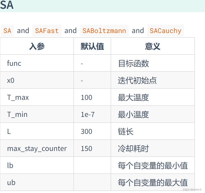
3.模拟退火(SA)

demo_func = lambda x: x[0] ** 2 + (x[1] - 0.05) ** 2 + x[2] ** 2

# %% Do SA
from sko.SA import SA

sa = SA(func=demo_func, x0=[1, 1, 1], T_max=1, T_min=1e-9, L=300, max_stay_counter=150)
best_x, best_y = sa.run()
print('best_x:', best_x, 'best_y', best_y)

# %% Plot the result
import matplotlib.pyplot as plt
import pandas as pd

plt.plot(pd.DataFrame(sa.best_y_history).cummin(axis=0))
plt.show()

# %%
from sko.SA import SAFast

sa_fast = SAFast(func=demo_func, x0=[1, 1, 1], T_max=1, T_min=1e-9, q=0.99, L=300, max_stay_counter=150)
sa_fast.run()
print('Fast Simulated Annealing: best_x is ', sa_fast.best_x, 'best_y is ', sa_fast.best_y)

# %%
from sko.SA import SAFast

sa_fast = SAFast(func=demo_func, x0=[1, 1, 1], T_max=1, T_min=1e-9, q=0.99, L=300, max_stay_counter=150,
                 lb=[-1, 1, -1], ub=[2, 3, 4])
sa_fast.run()
print('Fast Simulated Annealing with bounds: best_x is ', sa_fast.best_x, 'best_y is ', sa_fast.best_y)

# %%
from sko.SA import SABoltzmann

sa_boltzmann = SABoltzmann(func=demo_func, x0=[1, 1, 1], T_max=1, T_min=1e-9, q=0.99, L=300, max_stay_counter=150)
sa_boltzmann.run()
print('Boltzmann Simulated Annealing: best_x is ', sa_boltzmann.best_x, 'best_y is ', sa_fast.best_y)


# %%
from sko.SA import SABoltzmann

sa_boltzmann = SABoltzmann(func=demo_func, x0=[1, 1, 1], T_max=1, T_min=1e-9, q=0.99, L=300, max_stay_counter=150,
                           lb=-1, ub=[2, 3, 4])
sa_boltzmann.run()
print('Boltzmann Simulated Annealing with bounds: best_x is ', sa_boltzmann.best_x, 'best_y is ', sa_fast.best_y)

# %%
from sko.SA import SACauchy

sa_cauchy = SACauchy(func=demo_func, x0=[1, 1, 1], T_max=1, T_min=1e-9, q=0.99, L=300, max_stay_counter=150)
sa_cauchy.run()
print('Cauchy Simulated Annealing: best_x is ', sa_cauchy.best_x, 'best_y is ', sa_cauchy.best_y)

# %%
from sko.SA import SACauchy

sa_cauchy = SACauchy(func=demo_func, x0=[1, 1, 1], T_max=1, T_min=1e-9, q=0.99, L=300, max_stay_counter=150,
                     lb=[-1, 1, -1], ub=[2, 3, 4])
sa_cauchy.run()
print('Cauchy Simulated Annealing with bounds: best_x is ', sa_cauchy.best_x, 'best_y is ', sa_cauchy.best_y)

参数说明

---

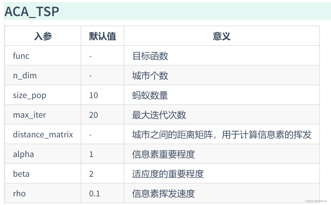
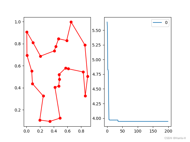
4.蚁群算法(ACA)

import numpy as np
from scipy import spatial
import pandas as pd
import matplotlib.pyplot as plt

num_points = 25

points_coordinate = np.random.rand(num_points, 2)  # generate coordinate of points
distance_matrix = spatial.distance.cdist(points_coordinate, points_coordinate, metric='euclidean')


def cal_total_distance(routine):
    num_points, = routine.shape
    return sum([distance_matrix[routine[i % num_points], routine[(i + 1) % num_points]] for i in range(num_points)])


# %% Do ACA
from sko.ACA import ACA_TSP

aca = ACA_TSP(func=cal_total_distance, n_dim=num_points,
              size_pop=50, max_iter=200,
              distance_matrix=distance_matrix)

best_x, best_y = aca.run()

# %% Plot
fig, ax = plt.subplots(1, 2)
best_points_ = np.concatenate([best_x, [best_x[0]]])
print(best_x)  # 结果序列
print(best_points_)  # 添加起点形成环
best_points_coordinate = points_coordinate[best_points_, :]  # 找到点序列对应的坐标序列
ax[0].plot(best_points_coordinate[:, 0], best_points_coordinate[:, 1], 'o-r')  # 连接
pd.DataFrame(aca.y_best_history).cummin().plot(ax=ax[1])
plt.show()

---

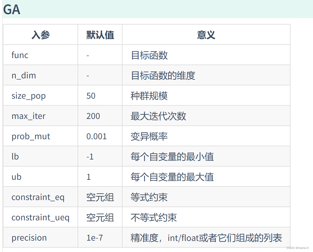
5.遗传算法(GA)

import numpy as np


def schaffer(p):
    '''
    This function has plenty of local minimum, with strong shocks
    global minimum at (0,0) with value 0
    https://en.wikipedia.org/wiki/Test_functions_for_optimization
    '''
    x1, x2 = p
    part1 = np.square(x1) - np.square(x2)
    part2 = np.square(x1) + np.square(x2)
    return 0.5 + (np.square(np.sin(part1)) - 0.5) / np.square(1 + 0.001 * part2)


# %%
from sko.GA import GA

ga = GA(func=schaffer, n_dim=2, size_pop=50, max_iter=800, prob_mut=0.001, lb=[-1, -1], ub=[1, 1], precision=1e-7)
best_x, best_y = ga.run()
print('best_x:', best_x, '\n', 'best_y:', best_y)
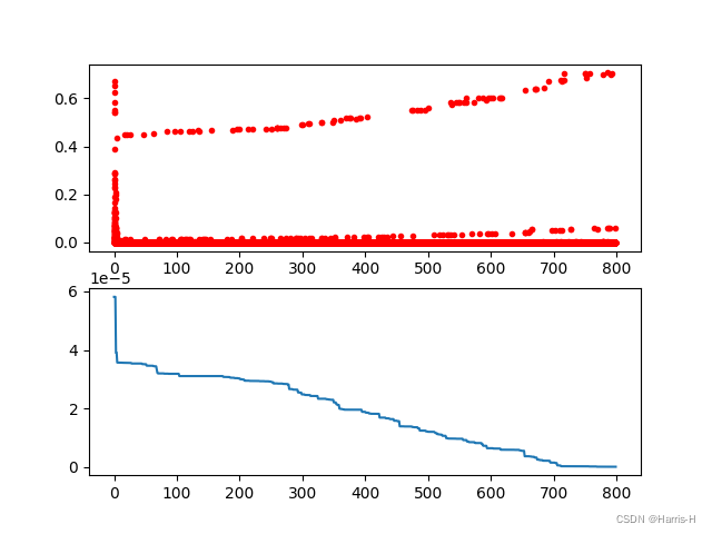
# %% Plot the result
import pandas as pd
import matplotlib.pyplot as plt

Y_history = pd.DataFrame(ga.all_history_Y)
print(Y_history)
fig, ax = plt.subplots(2, 1)
ax[0].plot(Y_history.index, Y_history.values, '.', color='red')
Y_history.min(axis=1).cummin().plot(kind='line')
plt.show()

结果

best_x: [0.00294498 0.00016674] 
 best_y: [8.77542544e-09]
               0             1   ...            48            49
0    2.432570e-01  8.702831e-02  ...  3.420108e-04  1.928273e-02
1    6.365298e-02  4.969987e-02  ...  1.994070e-02  3.016882e-02
2    8.110868e-04  5.950608e-04  ...  1.694919e-03  2.924401e-02
3    9.968317e-04  1.167487e-04  ...  1.288323e-03  2.983435e-04
4    2.318954e-03  2.191508e-04  ...  1.501895e-04  1.733578e-03
..            ...           ...  ...           ...           ...
795  9.406647e-09  8.849707e-09  ...  9.312904e-09  9.406647e-09
796  8.849707e-09  8.849707e-09  ...  8.830077e-09  8.849707e-09
797  8.849707e-09  8.849707e-09  ...  8.849707e-09  8.849707e-09
798  8.830077e-09  8.849707e-09  ...  8.849707e-09  8.849707e-09
799  8.830077e-09  8.849707e-09  ...  8.958900e-09  8.849707e-09

[800 rows x 50 columns]