


1.引言
手写数字是人手书写的各种字符中最简单常见的一种。在过去的30多年间,对手写数字识别的研究一直都是模式识别领域的研究热点。数字是世界各国通用的符号,类别也较少,有助于做深入分析及验证一些新的理论,因此它也是各种识别算法优劣的重要检测手段。手写数字识别的基本过程,一般可分为手写数字样本的收集、输入和预处理、特征提取、分类和识别等几个步骤。多年来,为了提高识别率和运行速度、降低误识率,众多的学者就纷纷识别的步骤提出各种新技术和新想法。大家讨论的焦点主要集中在特征提取、分类以及识别等方面。
手写数字识别(Handwritten Numeral Recognition)是光学字符识别技术(Optical Character Recogmition,简称OCR)的一个分支,它研究的对象是:如何利用电子计算机自动辨认人手写在纸张上的阿拉伯数字。随着社会信息化的发展,手写数字的识别研究有着重大的实用价值,如在邮政编码、税务报表、统计报表、财务报表、银行票据、海关、人口普查等需要处理大量字符信息录入的场合。
手写体数字识别方法大体可分为两类:基于统计的识别方法和基于结构的识别方法。第一类方法包括模板匹配法、矩法、笔道的点密度测试、字符轨迹法及数字变换法等。第二类则是尽量抽取数字的骨架或轮廓特征,如环路、端点、交叉点、弧状线、环及凹凸性等,两类方法具有一定的互补性。手写数字识别是当前图像处理和模式识别领域的一个重要研究分支,由于手写数字的随意性大,其识别准确率易受字体大小、笔画粗细和倾斜角度等因素的影响,因此进行手写数字识别方法和系统的设计具有重要的理论价值和实际意义。
手写体数字用多层BP网络来识别可以采用两种输入网络的形式:一种是点阵(0,1点阵)直接输入网络,利用网络来抽取特征并进行分类,这也叫点阵输入网络;另一种是通过一些算法,抽取字符特征,然后将一组特征值输入网络,利用神经网络对特征分类,达到识别字符的目的,这也叫作特征输入网络,它仅起分类作用。对于识别手写体数字,特征输入网络要比点阵输入网络效果好。
特征输入网络多数是直接输入提取的所有字符特征,一般来说,特征输入的越多识别才能越准确。但是太多的输入会使网络变的很大,难于收敛或者收敛到局部极小点。可以先对待识别数字进行粗特征分类,其作用是根据一些简单的特征对数字分类,选择具有这些简单特征的数字准备进行进一步识别;然后再提取其他特征,输入粗分类中选中的数字判别网络进行判别。
常用的特征提取方法,有逐像素特征提取法、骨架特征提取法和垂直方向数据统计特征提取法L6j等。逐像素特征提取法n3是一种最简单的特征提取方法,它是对图像进行逐行逐列地扫描,其特点是算法简单,运算速度快,可以使网络很快地收敛,训练效果好,但适应性不强;骨架特征提取法是一种利用细化的方法来提取骨架的方法。该方法对于线条粗细不同的数字有一定的适应性,但是图像一旦出现偏移就难以识别;垂直方向数据统计特征提取法就是自左向右对图像进行逐列地扫描,统计每列黑像素的个数,然后自上而下逐行扫描,统计每行的黑像素的个数,将统计结果作为字符的特征向量。这种方法的效果不是很理想,适应性不强。分类与识别的方式主要有贝叶斯分类器嘲、人工神经网络、多分类器组合或多级分类器、基于图论原理的分类、支持向量机等。由于人工神经网络具有自学习、容错性、分类能力强和并行处理等特点,因此它也是最常用的分类识别方式。在训练神经网络时最常用的是BP算法。由于手写体存在本身的不规则性及不同人书写风格的差异,手写数字的特征向量常出现交叉和混淆。可是BP网络采用剧变的判别边界来分割特征空间,对于样本特征空间存在交叉的情况,它将无法正确的估计出处于特征空间交叉处样本的隶属度值。不过,由于量子神经网络,具有超高速、超并行、指数容量级的特点,对具有不确定性、两类模式之间存在交叉数据的模式识别问题有极好的分类效果,因此,量子神经网络就可很好的克服常规BP神经网络的局限性。本文针对上述特征提取方法和BP神经网路的缺陷,提出了一种将新型特征提取方法(13维特征提取法)与量子神经网络相结合的手写数字识别方法。实验结果表明,与其他方法相比,该方法的识别正确率有了明显的提高。
3 全连接神经网络(DNN)
3.1全连接神经网络原理
全连接神经网络(DNN)是最朴素的神经网络,它的网络参数最多,计算量最大。
全连接神经网络规则如下:
-
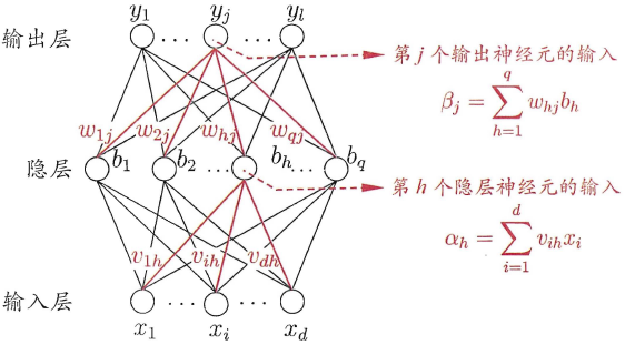
神经元按照层来布局。最左边的层叫做输入层,负责接收输入数据;最右边的层叫输出层,我们可以从这层获取神经网络输出数据。输入层和输出层之间的层叫做隐藏层,因为它们对于外部来说是不可见的。
-
同一层的神经元之间没有连接。
-
第N层的每个神经元和第N-1层的所有神经元相连(这就是full connected的含义),第N-1层神经元的输出就是第N层神经元的输入。
-
每个连接都有一个权值。
DNN的结构不固定,一般神经网络包括输入层、隐藏层和输出层,一个DNN结构只有一个输入层,一个输出层,输入层和输出层之间的都是隐藏层。每一层神经网络有若干神经元,层与层之间神经元相互连接,层内神经元互不连接,而且下一层神经元连接上一层所有的神经元。
隐藏层比较多(>2)的神经网络叫做深度神经网络(DNN的网络层数不包括输入层),深度神经网络的表达力比浅层网络更强,一个仅有一个隐含层的神经网络就能拟合任何一个函数,但是它需要很多很多的神经元。
优点:由于DNN几乎可以拟合任何函数,所以DNN的非线性拟合能力非常强。往往深而窄的网络要更节约资源。
缺点:DNN不太容易训练,需要大量的数据,很多技巧才能训练好一个深层网络。
感知器
DNN也可以叫做多层感知器(MLP),DNN的网络结构太复杂,神经元数量太多,为了方便讲解我们设计一个最简单的DNN网络结构--感知机
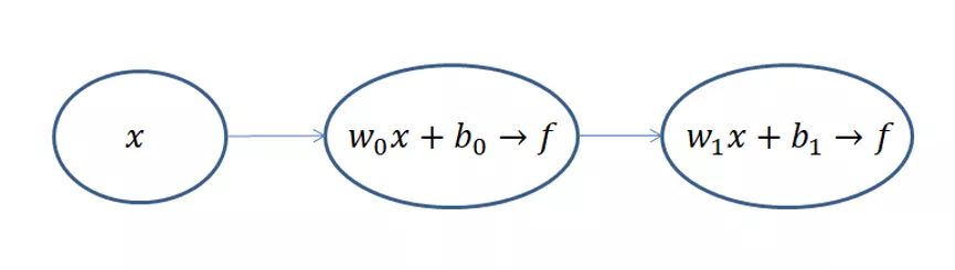
这是一个只有两层的神经网络,假定输入
x
x
x,我们规定隐层h和输出层o这两层都是
z
=
w
x
+
b
z=wx+b
z=wx+b和
f
(
z
)
=
1
1
+
e
−
z
f(z)=\frac{1}{1+e^{-z}}
f(z)=1+e−z1的组合,一旦输入样本x和标签y之后,模型就开始训练了。那么我们的问题就变成了求隐藏层的
w
0
、
b
0
w_0、b_0
w0、b0和输出层的
w
1
、
b
1
w_1、b_1
w1、b1四个参数的过程。
训练的目的是神经网络的输出和真实数据的输出"一样",但是在"一样"之前,模型输出和真实数据都是存在一定的差异,我们把这个"差异"作这样的一个参数 e e e代表误差的意思,那么模型输出加上误差之后就等于真实标签了,作: y = w x + b + e y=wx+b+e y=wx+b+e
当我们有n对 x x x和 y y y那么就有n个误差 e e e,我们试着把n个误差 e e e都加起来表示一个误差总量,为了不让残差正负抵消我们取平方或者取绝对值,本文取平方。这种误差我们称为“残差”,也就是模型的输出的结果和真实结果之间的差值。损失函数Loss还有一种称呼叫做“代价函数Cost”,残差表达式如下:
L o s s = ∑ i = 1 n e i 2 = ∑ i = 1 n ( y i − ( w x i + b ) ) 2 Loss=\sum_{i=1}^{n}e_i^2=\sum_{i=1}^{n}(y_i-(wx_i+b))^2 Loss=i=1∑nei2=i=1∑n(yi−(wxi+b))2
现在我们要做的就是找到一个比较好的w和b,使得整个Loss尽可能的小,越小说明我们训练出来的模型越好。
反向传播算法(BP)
BP算法主要有以下三个步骤 :
- 前向计算每个神经元的输出值;
- 反向计算每个神经元的误差项 e e e值;
- 最后用随机梯度下降算法迭代更新权重w和b。
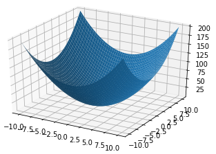
我们把损失函数展开如下图所示,他的图形到底长什么样子呢?到底该怎么求他的最小值呢?
\begin{eqnarray}
Loss&=&\sum_{i=1}{n}(x_i2w2+b2+2x_iwb-2y_ib-2x_iy_iw+y_i^2)\
&=&Aw2+Bb2+Cwb+Db+Dw+Eb+F
\end{eqnarray}
我们初始化一个
w
0
w_0
w0和
b
0
b_0
b0,带到Loss函数里面去,这个点(
w
o
,
b
o
,
L
o
s
s
o
w_o,b_o,Loss_o
wo,bo,Losso)会出现在碗壁的某个位置,而我们的目标位置是碗底,那就慢慢的一点一点的往底部挪吧。
x n + 1 = x n − η d f ( x ) d x x_{n+1}=x_n-\eta \frac{df(x)}{dx} xn+1=xn−ηdxdf(x)
上式为梯度下降算法的公式,其中 d f ( x ) d x \frac{df(x)}{dx} dxdf(x)为梯度, η \eta η是学习率,也就是每次挪动的步长, η \eta η大每次迭代的脚步就大, η \eta η小每次迭代的脚步就小,我们只有取到合适的 η \eta η才能尽可能的接近最小值而不会因为步子太大越过了最小值。
当 x n = 3 x_n=3 xn=3时, − η d f ( x ) d x -\eta\frac{df(x)}{dx} −ηdxdf(x)为负数,更新后 x n + 1 x_{n+1} xn+1会减小;当 x n = − 3 x_n=-3 xn=−3时, − η d f ( x ) d x -\eta\frac{df(x)}{dx} −ηdxdf(x)为正数,更新后 x n + 1 x_{n+1} xn+1还是会减小。这总函数其实就是凸函数。满足 f ( x i + x 2 2 ) = f ( x i ) + f ( x 2 ) 2 f(\frac{x_i+x_2}{2})=\frac{f(x_i)+f(x_2)}{2} f(2xi+x2)=2f(xi)+f(x2)都是凸函数。沿着梯度的方向是下降最快的。
我们初始化 ( w 0 , b 0 , L o s s o ) (w_0,b_0,Loss_o) (w0,b0,Losso)后下一步就水到渠成了,
w 1 = w o − η ∂ L o s s ∂ w , b 1 = b o − η ∂ L o s s ∂ b w_1=w_o-\eta \frac{\partial Loss}{\partial w},b_1=b_o-\eta \frac{\partial Loss}{\partial b} w1=wo−η∂w∂Loss,b1=bo−η∂b∂Loss
有了梯度和学习率 η \eta η乘积之后,当这个点逐渐接近“碗底”的时候,偏导也随之下降,移动步伐也会慢慢变小,收敛会更为平缓,不会轻易出现“步子太大”而越过最低的情况。一轮一轮迭代,但损失值的变化趋于平稳时,模型的差不多就训练完成了。
梯度下降算法
我们用 w n e w = w o l d − η ∂ L o s s ∂ w w_{new}=w_{old}-\eta\frac{\partial Loss}{\partial w} wnew=wold−η∂w∂Loss讲以下梯度下降算法,零基础的读者可以仔细观看,有基础的请忽视梯度下降算法,我们定义y为真实值, y ^ \hat{y} y^为预测值
∂ L o s s ∂ w = ∂ ∂ w 1 2 ∑ i = 1 n ( y − y ^ ) 2 = 1 2 ∑ i = 1 n ∂ ∂ w ( y − y ^ ) 2 \frac{\partial Loss}{\partial w}=\frac{\partial}{\partial\mathrm{w}}\frac{1}{2}\sum_{i=1}^{n}(y-\hat{y})^2=\frac{1}{2}\sum_{i=1}^{n}\frac{\partial}{\partial\mathrm{w}}(y-\hat{y})^2 ∂w∂Loss=∂w∂21i=1∑n(y−y^)2=21i=1∑n∂w∂(y−y^)2
y是与 w w w无关的参数,而 y ^ = w x + b \hat{y}=wx+b y^=wx+b,下面我们用复合函数求导法
∂ L o s s ∂ w = ∂ L o s s ∂ y ^ ∂ y ^ ∂ w \frac{\partial Loss}{\partial\mathrm{w}}=\frac{\partial Loss}{\partial \hat{y}} \frac{\partial \hat{y}}{\partial w} ∂w∂Loss=∂y^∂Loss∂w∂y^
分别计算上式等号右边的两个偏导数
∂ L o s s ∂ y ^ = ∂ ∂ y ^ ( y 2 − 2 y y ^ + y ^ 2 ) = − 2 y + 2 y ^ \frac{\partial Loss}{\partial\hat{y}}=\frac{\partial}{\partial \hat{y}}(y^2-2y\hat{y}+\hat{y}^2)=-2y+2\hat{y} ∂y^∂Loss=∂y^∂(y2−2yy^+y^2)=−2y+2y^
∂ y ^ ∂ w = ∂ ∂ w ( w x + b ) = x \frac{\partial \hat{y}}{\partial\mathrm{w}}=\frac{\partial}{\partial\mathrm{w}}(wx+b)=x ∂w∂y^=∂w∂(wx+b)=x
代入 ∂ L o s s ∂ w \frac{\partial Loss}{\partial w} ∂w∂Loss,求得
∂ L o s s ∂ w = 1 2 ∑ i = 1 n ∂ ∂ w ( y − y ^ ) 2 = 1 2 ∑ i = 1 n 2 ( − y + y ^ ) x = − ∑ i = 1 n ( y − y ^ ) x \frac{\partial Loss}{\partial\mathrm{w}}=\frac{1}{2}\sum_{i=1}^{n}\frac{\partial}{\partial\mathrm{w}}(y-\hat{y})^2=\frac{1}{2}\sum_{i=1}^{n}2(-y+\hat{y})\mathrm{x}=-\sum_{i=1}^{n}(y-\hat{y})\mathrm{x} ∂w∂Loss=21i=1∑n∂w∂(y−y^)2=21i=1∑n2(−y+y^)x=−i=1∑n(y−y^)x
有了上面的式字,我们就能写出训练线性单元的代码
[ w 0 w 1 w 2 … w m ] n e w = [ w 0 w 1 w 2 … w m ] o l d + η ∑ i = 1 n ( y − y ^ ) [ x 0 x 1 x 2 … x m ] \begin{bmatrix} w_0 \\ w_1 \\ w_2 \\ … \\ w_m \\ \end{bmatrix}_{new}= \begin{bmatrix} w_0 \\ w_1 \\ w_2 \\ … \\ w_m \\ \end{bmatrix}_{old}+\eta\sum_{i=1}^{n}(y-\hat{y}) \begin{bmatrix} x_0 \\ x_1\\ x_2\\ … \\ x_m\\ \end{bmatrix} ⎣ ⎡w0w1w2…wm⎦ ⎤new=⎣ ⎡w0w1w2…wm⎦ ⎤old+ηi=1∑n(y−y^)⎣ ⎡x0x1x2…xm⎦ ⎤

这个网络用函数表达式写的话如下所示:
第一层(隐藏层) z h = w n x + b n , y h = 1 1 + e − z h \begin{matrix}z_h=w_nx+b_n,&y_h=\frac{1}{1+e^{-z_h}}\end{matrix} zh=wnx+bn,yh=1+e−zh1
第二层(输出层) z o = w o y h + b o , y o = 1 1 + e − z o \begin{matrix}z_o=w_oy_h+b_o,&y_o=\frac{1}{1+e^{-z_o}}\end{matrix} zo=woyh+bo,yo=1+e−zo1
接下来的工作就是把 w h 、 b h 、 w o 、 b o w_h、b_h、w_o、b_o wh、bh、wo、bo参数利用梯度下降算法求出来,把损失函数降低到最小,那么我们的模型就训练出来呢。
第一步:准备样本,每一个样本 x i x_i xi对应标签 y i y_i yi。
第二步:清洗数据,清洗数据的目的是为了帮助网络更高效、更准确地做好分类。
第三步:开始训练,
L o s s = ∑ i = 1 n ( y o i − y i ) 2 Loss=\sum_{i=1}^{n}(y_{oi}-y_i)^2 Loss=i=1∑n(yoi−yi)2
我们用这四个表达式,来更新参数。
( w h ) n = ( w h ) n − 1 − η ∂ L o s s ∂ w h (w_h)^n=(w_h)^{n-1}-\eta \frac{\partial Loss}{\partial w_h} (wh)n=(wh)n−1−η∂wh∂Loss
( b h ) n = ( b h ) n − 1 − η ∂ L o s s ∂ b h (b_h)^n=(b_h)^{n-1}-\eta \frac{\partial Loss}{\partial b_h} (bh)n=(bh)n−1−η∂bh∂Loss
( w o ) n = ( w o ) n − 1 − η ∂ L o s s ∂ w o (w_o)^n=(w_o)^{n-1}-\eta \frac{\partial Loss}{\partial w_o} (wo)n=(wo)n−1−η∂wo∂Loss
( b o ) n = ( b o ) n − 1 − η ∂ L o s s ∂ b o (b_o)^n=(b_o)^{n-1}-\eta \frac{\partial Loss}{\partial b_o} (bo)n=(bo)n−1−η∂bo∂Loss
问题来了, ∂ L o s s ∂ w h \frac{\partial Loss}{\partial w_h} ∂wh∂Loss、 ∂ L o s s ∂ b h \frac{\partial Loss}{\partial b_h} ∂bh∂Loss、 ∂ L o s s ∂ w o \frac{\partial Loss}{\partial w_o} ∂wo∂Loss、 ∂ L o s s ∂ b o \frac{\partial Loss}{\partial b_o} ∂bo∂Loss这4个值怎么求呢?
L o s s = ∑ i = 1 n ( y o i − y i ) 2 ⇒ L o s s = 1 2 ∑ i = 1 n ( y o i − y i ) 2 Loss=\sum_{i=1}^{n}(y_{oi}-y_i)^2\Rightarrow Loss=\frac{1}{2}\sum_{i=1}^{n}(y_{oi}-y_i)^2 Loss=i=1∑n(yoi−yi)2⇒Loss=21i=1∑n(yoi−yi)2
配一个 1 2 \frac{1}{2} 21出来,为了后面方便化简。
∂ L o s s ∂ w h = ∂ ∑ i = 1 n 1 2 ( y o i − y i ) 2 ∂ w o = ∂ ∑ i = 1 n y o i w o = ∑ i = 1 n ∂ y o i ∂ z o ⋅ z o w o = ∑ i = 1 n ∂ y o i ∂ z o ⋅ z o y h ⋅ ∂ y h ∂ z h ⋅ ∂ z h ∂ w h \frac{\partial Loss}{\partial w_h}=\frac{\partial \sum_{i=1}^{n}\frac{1}{2}(y_{oi}-y_i)^2}{\partial w_o}=\frac{\partial \sum_{i=1}^{n}y_{oi}}{w_o}=\sum_{i=1}^{n}\frac{\partial y_{oi}}{\partial z_o}·\frac{z_o}{w_o}=\sum_{i=1}^{n}\frac{\partial y_{oi}}{\partial z_o}·\frac{z_o}{y_h}·\frac{\partial y_h}{\partial z_h}·\frac{\partial z_h}{\partial w_h} ∂wh∂Loss=∂wo∂∑i=1n21(yoi−yi)2=wo∂∑i=1nyoi=i=1∑n∂zo∂yoi⋅wozo=i=1∑n∂zo∂yoi⋅yhzo⋅∂zh∂yh⋅∂wh∂zh
其他三个参数,和上面类似,这是一种“链乘型”求导方式。我们的网络两层就4个连乘,如果是10层,那么就是20个连乘。但一层网络的其中一个节点连接着下一层的其他节点时,那么这个节点上的系数的偏导就会通过多个路径传播过去,从而形成“嵌套型关系”。
DropOut
DropOut是深度学习中常用的方法,主要是为了克服过拟合的现象。全连接网络极高的VC维,使得它的记忆能力非常强,甚至把一下无关紧要的细枝末节都记住,一来使得网络的参数过多过大,二来这样训练出来的模型容易过拟合。
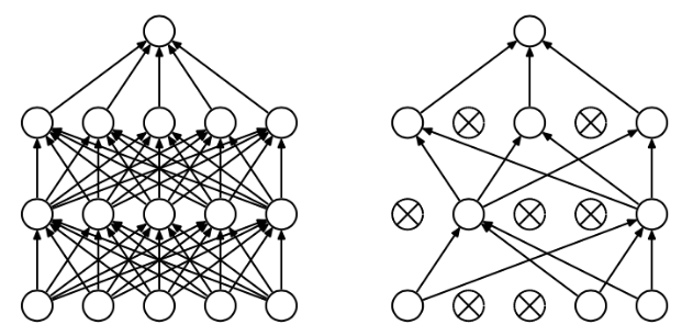
DropOut:是指在在一轮训练阶段临时关闭一部分网络节点。让这些关闭的节点相当去去掉。如下图所示去掉虚线圆和虚线,原则上是去掉的神经元是随机的。
python代码实现
** 手写数字是通过矩阵录入电脑的,我们先来研究一下怎么将数字图片变为矩阵**
from PIL import Image

im = Image.open('D:\\Download\\5.png')  # 图像路径
width = im.size[0]
height = im.size[1]

fh = open('1.txt','w')  # 转换成的txt文件

for i in range(height):
    for j in range(width):
        # 获取像素点颜色
        color = im.getpixel((j,i))
        # 如果color=0则说明是黑色,写成1;如果color=1则说明是白色,写成0
        if(color == 0):
            fh.write('1')
        else:
            fh.write('0')
    fh.write('\n')
fh.close()
我们来查看第一个测试数据的输入
import tensorflow as tf  # 深度学习库,Tensor 就是多维数组

mnist = tf.contrib.keras.datasets.mnist  # mnist 是 28x28 的手写数字图片和对应标签的数据集
(x_train, y_train),(x_test, y_test) = mnist.load_data()  # 分割数据集
print(x_train[0]) # 查看第一个测试数据的输入
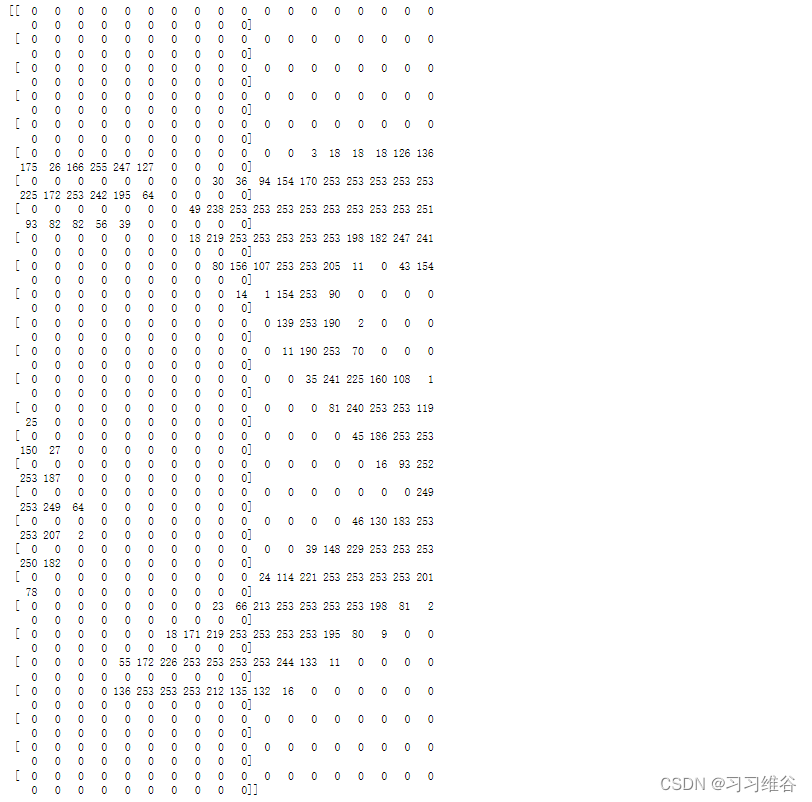
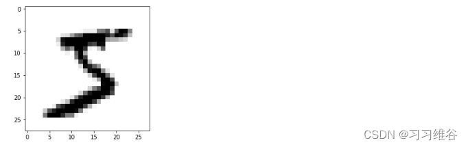
让我们把这个矩阵用图像表示出来
import matplotlib.pyplot as plt
%matplotlib inline
plt.imshow(x_train[0],cmap=plt.cm.binary) # 显示黑白图像
plt.show()
单层线性神经网络
现在我们知道了怎么进行手写数字和矩阵的转换
让我们先研究一个最简单的线性神经网络
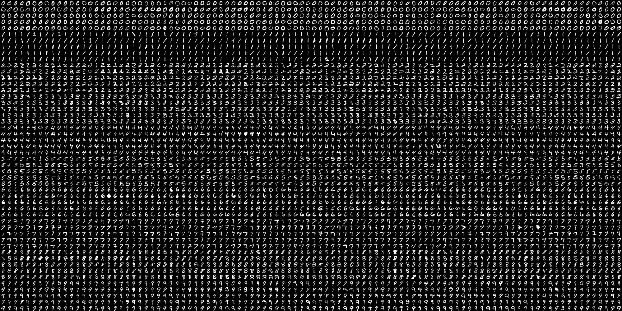
所用到的手写数据集是已经录入处理好的数据集MNIST
- 训练迭代次数
from __future__ import absolute_import
from __future__ import division
from __future__ import print_function
import tensorflow as tf
from tensorflow.examples.tutorials.mnist import input_data
import numpy as np
import matplotlib.pyplot as plt
# Import data
#下载和读取MNIST的训练集、测试集和验证集
#将数据读到内存后,我们就可以直接通过mnist.test.images和mnist.test.labels来获得测试集的图片和对应的标签了。TensorFlow提供的方法从训练集里取了5000个样本作为验证集,所以训练集、测试集、验证集的大小分别为:55000、10000、5000。
#'input_data/'是你存放下载的数据集的文件夹名。
mnist = input_data.read_data_sets('input_data/', one_hot=True)
# Create the model
x = tf.placeholder(tf.float32, [None, 784])
#这里简单的将参数都初始化为0。在复杂的模型中,初始化参数有很多的技巧。
W = tf.Variable(tf.zeros([784, 10]))
b = tf.Variable(tf.zeros([10]))
#一个简单的线性模型,tf.matmul表示矩阵相乘。
y = tf.matmul(x, W) + b
y_ = tf.placeholder(tf.float32, [None, 10])
keep_prob = tf.placeholder("float")
#计算每个样本的cross-entropy
# loss function & optimization algorithm
cross_entropy = tf.reduce_mean(tf.nn.softmax_cross_entropy_with_logits(labels=y_, logits=y))
train_step = tf.train.AdamOptimizer(1e-4).minimize(cross_entropy)
sess = tf.InteractiveSession()
tf.global_variables_initializer().run()
losss = []
accurs = []
steps = []
correct_predict = tf.equal(tf.argmax(y, 1), tf.argmax(y_, 1))
accuracy = tf.reduce_mean(tf.cast(correct_predict, tf.float32))
for i in range(20000):
batch = mnist.train.next_batch(50)
sess.run(train_step, feed_dict={x: batch[0], y_: batch[1], keep_prob: 0.5})
if i % 100 == 0:
loss = sess.run(cross_entropy, {x: batch[0], y_: batch[1], keep_prob: 1.0})
accur = sess.run(accuracy, feed_dict={x: mnist.test.images, y_: mnist.test.labels, keep_prob: 1.0})
steps.append(i)
losss.append(loss)
accurs.append(accur)
# plot loss
plt.figure()
plt.plot(steps, losss)
plt.xlabel('Number of steps')
plt.ylabel('Loss')
plt.figure()
plt.plot(steps, accurs)
plt.hlines(0.92, 0, max(steps), colors='r', linestyles='dashed')
plt.xlabel('Number of steps')
plt.ylabel('Accuracy')
plt.show()
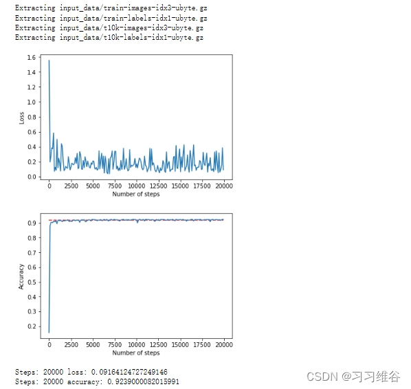
print('Steps: {} loss: {}'.format(20000, loss))
print('Steps: {} accuracy: {}'.format(20000, accur))
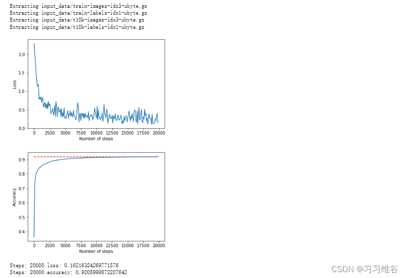
可以看到,我们最终的准确率大约在0.92左右,在上面模型中优化器使用Adam,学习率设为1e-4。我们可以考虑换一个优化器(梯度下降法)来求损失函数。
- 不同的优化器
from __future__ import absolute_import
from __future__ import division
from __future__ import print_function

import tensorflow as tf
from tensorflow.examples.tutorials.mnist import input_data
import numpy as np
import matplotlib.pyplot as plt

# Import data
#下载和读取MNIST的训练集、测试集和验证集
#将数据读到内存后,我们就可以直接通过mnist.test.images和mnist.test.labels来获得测试集的图片和对应的标签了。TensorFlow提供的方法从训练集里取了5000个样本作为验证集,所以训练集、测试集、验证集的大小分别为:55000、10000、5000。
#'input_data/'是你存放下载的数据集的文件夹名。
mnist = input_data.read_data_sets('input_data/', one_hot=True)

# Create the model
x = tf.placeholder(tf.float32, [None, 784])
#这里简单的将参数都初始化为0。在复杂的模型中,初始化参数有很多的技巧。
W = tf.Variable(tf.zeros([784, 10]))
b = tf.Variable(tf.zeros([10]))
#一个简单的线性模型,tf.matmul表示矩阵相乘。
y = tf.matmul(x, W) + b
y_ = tf.placeholder(tf.float32, [None, 10])
keep_prob = tf.placeholder("float")
#计算每个样本的cross-entropy
# loss function & optimization algorithm
cross_entropy = tf.reduce_mean(tf.nn.softmax_cross_entropy_with_logits(labels=y_, logits=y))
train_step = tf.train.GradientDescentOptimizer(0.5).minimize(cross_entropy)
sess = tf.InteractiveSession()
tf.global_variables_initializer().run()

losss = []
accurs = []
steps = []
correct_predict = tf.equal(tf.argmax(y, 1), tf.argmax(y_, 1))
accuracy = tf.reduce_mean(tf.cast(correct_predict, tf.float32))
for i in range(20000):
    batch = mnist.train.next_batch(50)
    sess.run(train_step, feed_dict={x: batch[0], y_: batch[1], keep_prob: 0.5})

    if i % 100 == 0:
        loss = sess.run(cross_entropy, {x: batch[0], y_: batch[1], keep_prob: 1.0})
        accur = sess.run(accuracy, feed_dict={x: mnist.test.images, y_: mnist.test.labels, keep_prob: 1.0})
        steps.append(i)
        losss.append(loss)
        accurs.append(accur)

# plot loss
plt.figure()
plt.plot(steps, losss)
plt.xlabel('Number of steps')
plt.ylabel('Loss')

plt.figure()
plt.plot(steps, accurs)
plt.hlines(0.92, 0, max(steps), colors='r', linestyles='dashed')
plt.xlabel('Number of steps')
plt.ylabel('Accuracy')
plt.show()

print('Steps: {} loss: {}'.format(20000, loss))
print('Steps: {} accuracy: {}'.format(20000, accur))
结论:单层的Softmax Regression进行手写数字识别的准确率约为92%,比传统机器学习的预测效果还是差很多的,不过这只是最简单的线性神经网络,所以我们可以继续继续探究
二层神经网络
神经网络设计
将28×28的图片转换成向量,长度为784,因此神经网络的输入层有784个神经元;输出层显然需要10个神经元,因为输出的是0~9这10个数字;隐含层采用15个神经元。网络结构如下:

- 隐层的激活函数采用 sigmoid 函数,输出层的激活函数采用 softmax 函数。
- 损失函数为实际的label与概率归一化预测输出的交叉熵,具体采用 “tf.nn.softmax_cross_entropy_with_logits” 进行计算
- 优化算法采用Adam算法,即tensorflow中的“tf.train.AdamOptimizer”。(因为之前的研究中发现不同优化器得出的准确度差不多,故此处不再另外画tf.train.GradientDescentOptimizer(梯度下降法)的结果图)
python代码
import os
os.environ['TF_CPP_MIN_LOG_LEVEL'] = '2'
old_v = tf.logging.get_verbosity()
tf.logging.set_verbosity(tf.logging.ERROR)

# create model
# input layer
x = tf.placeholder(tf.float32, [None, 784])  # input images
y_ = tf.placeholder(tf.float32, [None, 10])  # input labels

# hidden layer
hidden_layer_count = 15
w1 = tf.Variable(tf.zeros([784, hidden_layer_count]))
b1 = tf.Variable(tf.zeros([hidden_layer_count]))
y1 = tf.sigmoid(tf.matmul(x, w1) + b1)

# output layer
output_layer_count = 10
w2 = tf.Variable(tf.zeros([hidden_layer_count, output_layer_count]))
b2 = tf.Variable(tf.zeros(output_layer_count))
y2 = tf.nn.softmax(tf.matmul(y1, w2) + b2)

# loss function & optimization algorithm
cross_entropy = tf.reduce_mean(tf.nn.softmax_cross_entropy_with_logits(labels=y_, logits=y2))
train_step = tf.train.AdamOptimizer(learning_rate=0.01).minimize(cross_entropy)

# new session
sess = tf.Session()
sess.run(tf.global_variables_initializer())

# train
for i in range(10000):
    batch_xs, batch_ys = mnist.train.next_batch(50)
    sess.run(train_step, feed_dict={x: batch_xs, y_: batch_ys})
    if i % 1000 == 0:
        loss = sess.run(cross_entropy, {x: batch_xs, y_: batch_ys})
        print("Iter: %s loss: %s" % (i, loss))

# test
correct_prediction = tf.equal(tf.argmax(y_, 1), tf.argmax(y2, 1))
accuracy = tf.reduce_mean(tf.cast(correct_prediction, tf.float32))
print('Accuracy: ', sess.run(accuracy, feed_dict={x: mnist.test.images, y_: mnist.test.labels}))

tf.logging.set_verbosity(old_v)

该方法最终的准确率约为72.07%。使用单层的Softmax Regression进行手写数字识别的准确率约为92%,而加了一层隐层之后,准确率只有70%左右,令人感到意外,因为一般网络越深,分类效果应该越好才对。不过简单分析一下,原因可能就是加了一层隐层之后参数数量变大,容易产生过拟合等。单层的Softmax Regression网络其参数个数为78410+10=7850,而增加一层15个神经元的隐层之后,参数个数变为(78415+15)+(15*10+10)=11935。因此我们可以通过调整隐层神经元的个数、w和b的初始值、激活函数、学习率、每批训练样本的个数、训练的迭代次数等尝试提高准确率。
优化策略
一、指数衰减学习率
学习率是指每次参数更新的幅度,如下。
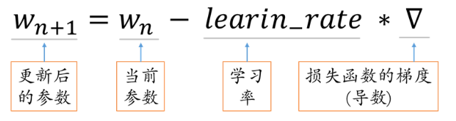
学习率设置的过小则参数更新太慢,学习效率低;学习率设置的太大,则后期容易产生振荡,难以收敛。但在参数更新前期,参数距离最优参数较远,希望学习率设置的大些;而在参数更新后期,参数距离最优参数较近,为了避免产生振荡,希望参数设置的小些。由此可见,学习率设置成固定值并不是最好的。
指数衰减学习率是根据运行的轮数动态调整学习率的一种方法,在TensorFlow中表示如下:
tf.train.exponential_decay(
    learning_rate,        # 学习率初始值
    global_step,          # 当前训练总轮数(不能为负)
    decay_steps,          # 衰减步长(必须为正),即多少轮更新一次学习率
    decay_rate,           # 衰减率,一般取值范围为(0,1)
    staircase=False,      # True:阶梯型衰减, False:平滑衰减
    name=None             # 操作的可选名称,默认为'ExponentialDecay'
)
学习率的计算公式为:
decayed_learning_rate = learning_rate *
                        decay_rate ^ (global_step / decay_steps)
注意当staircase为Ture时,global_step / decay_steps是一个整数,衰减率为阶梯函数 ,如下
import tensorflow as tf
import numpy as np
import matplotlib.pyplot as plt
%matplotlib inline

learning_rate = 0.5
decay_rate = 0.9
global_steps = 1000
decay_steps = 100

global_step = tf.Variable(0)
lr1 = tf.train.exponential_decay(
    learning_rate = learning_rate,
    global_step = global_step,
    decay_steps = decay_steps,
    decay_rate = decay_rate,
    staircase = True
)
lr2 = tf.train.exponential_decay(
    learning_rate = learning_rate,
    global_step = global_step,
    decay_steps = decay_steps,
    decay_rate = decay_rate,
    staircase = False
)

LR1 = []
LR2 = []
with tf.Session() as sess:
    for i in range(global_steps):
        LR1.append(sess.run(lr1, feed_dict = {global_step: i}))
        LR2.append(sess.run(lr2, feed_dict = {global_step: i}))

plt.figure(1)
plt.plot(range(global_steps), LR1, 'r-')
plt.plot(range(global_steps), LR2, 'b-')
plt.show()
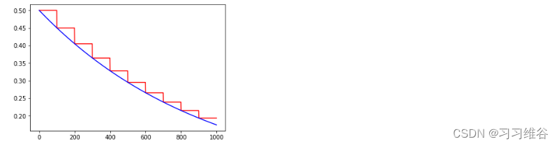
其中lr1的staircase =True, 而 lr2的staircase =False,衰减如下所示,lr1是红色曲线,lr2是蓝色曲线,可以看到lr1中每经过decay_steps = 100步之后进行计算,而lr2在每个step都进行计算。
二、正则化
当模型比较复杂时,它会去拟合数据中的噪声而损失了一定的通用性,即产生了过拟合。为了避免过拟合问题,常用的方法是加入正则化项,即在损失函数中加入刻画模型复杂程度的指标,将优化目标定义为 J ( θ ) + λ R ( w ) J(\theta)+λR(w) J(θ)+λR(w),其中R(w)刻画的是模型的复杂程度,包括了权重项w不包括偏置项b,λ表示模型复杂损失在总损失中的比例。
常用的正则化有L1正则化和L2正则化,
R
(
w
)
=
∣
∣
ω
∣
∣
1
=
∑
i
∣
∣
ω
∣
i
∣
R(w) = {||\omega||}_1 = \sum_{i}|{|\omega|}_i|
R(w)=∣∣ω∣∣1=i∑∣∣ω∣i∣
R
(
w
)
=
∣
∣
ω
∣
∣
2
2
=
∑
i
∣
∣
ω
∣
i
2
∣
R(w) = {||\omega||}_2^2 = \sum_{i}|{|\omega|}_i^2|
R(w)=∣∣ω∣∣22=i∑∣∣ω∣i2∣
其中,L1正则化会让参数变得更稀疏,L2则不会。一个含有L2正则化的损失函数的例子:
loss = tf.reduce_mean(tf.square(y_ - y)) + tf.contrib.layers.l2_regularizer(lambda)(w)
其中损失函数的第一项一般为预测输出和真实label之间的均方误差或交叉熵,第二项即为L2正则化项,lambda表示正则化项的权重,也就是J(θ)+λR(w)中的λ,w为需要计算正则化损失的参数。
TensorFlow中tf.contrib.layers.l2_regularizer函数的定义:
tf.contrib.layers.l2_regularizer(
    scale,  # 正则项的系数
    scope=None  # 可选的scope name
)
在简单的神经网络中,加入正则化来计算损失函数还是比较容易的。当神经网络变得非常复杂(层数很多)的时候,那么在损失函数中加入正则化的就会变得非常的复杂,使得损失函数的定义变得很长,从而还会导致程序的可读性变差,如这个例子。而且还有可能,当神经网络变得复杂的时候,定义网络结构的部分和计算损失函数的部分不在同一个函数中,这样就会使得计算损失函数不方便。TensorFlow提供了集合的方式,通过在计算图中保存一组实体,来解决这一类问题。
优化后
隐层神经元个数仍设为15个,隐层激活函数改为Relu函数。weight初始化为服从正态分布的随机数,bias初始化为常数0.1。
使用指数衰减学习率,学习率初始值设为0.01,衰减步长设为训练集的batch个数,衰减率设为0.99,优化算法采用Adam。
加入了正则化,正则项的系数设为0.0001。batch的大小为100,训练次数为20000,程序如下。
import tensorflow as tf
from tensorflow.examples.tutorials.mnist import input_data
import matplotlib.pyplot as plt

# move warning
import os
os.environ['TF_CPP_MIN_LOG_LEVEL'] = '2'
old_v = tf.logging.get_verbosity()
tf.logging.set_verbosity(tf.logging.ERROR)

# neural network parameters
INPUT_NODE = 784
LAYER1_NODE = 15
OUTPUT_NODE = 10

# exponential attenuation learning rate
LEARNING_RATE_BASE = 0.01
LEARNING_RATE_DECAY = 0.99

# regularization coefficient
LAMDA = 0.0001

# training parameters
BATCH_SIZE = 100
TRAINING_STEPS = 100000


# initialize weights and add regularization
def get_weight(shape, lamda):
    weights = tf.Variable(tf.random_normal(shape=shape), dtype=tf.float32)
    tf.add_to_collection("losses", tf.contrib.layers.l2_regularizer(lamda)(weights))
    return weights


# read data
mnist = input_data.read_data_sets('input_data/', one_hot=True)

# create model
# input layer
x = tf.placeholder(tf.float32, [None, INPUT_NODE])  # input images
y_ = tf.placeholder(tf.float32, [None, OUTPUT_NODE])  # input labels

# hidden layer
w1 = get_weight([INPUT_NODE, LAYER1_NODE], LAMDA)
b1 = tf.Variable(tf.constant(0.1, shape=[LAYER1_NODE]))
y1 = tf.nn.relu(tf.matmul(x, w1) + b1)

# output layer
w2 = get_weight([LAYER1_NODE, OUTPUT_NODE], LAMDA)
b2 = tf.Variable(tf.constant(0.1, shape=[OUTPUT_NODE]))
y2 = tf.nn.softmax(tf.matmul(y1, w2) + b2)

# loss function
cross_entropy = tf.reduce_mean(tf.nn.softmax_cross_entropy_with_logits(labels=y_, logits=y2))
tf.add_to_collection('losses', cross_entropy)
loss = tf.add_n(tf.get_collection('losses'))

# optimization algorithm
global_step = tf.Variable(0, trainable=False)
learning_rate = tf.train.exponential_decay(LEARNING_RATE_BASE, global_step,
                                           mnist.train.num_examples / BATCH_SIZE, LEARNING_RATE_DECAY)
train_step = tf.train.AdamOptimizer(learning_rate=learning_rate).minimize(loss, global_step=global_step)

# new session
sess = tf.Session()
sess.run(tf.global_variables_initializer())

# train
losss = []
accurs = []
steps = []
rates = []
correct_prediction = tf.equal(tf.argmax(y_, 1), tf.argmax(y2, 1))
accuracy = tf.reduce_mean(tf.cast(correct_prediction, tf.float32))
for i in range(TRAINING_STEPS):
    batch_xs, batch_ys = mnist.train.next_batch(BATCH_SIZE)
    _, now_loss, step, now_learn_rate = sess.run([train_step, loss, global_step, learning_rate],
                                                 feed_dict={x: batch_xs, y_: batch_ys})

    if i % 1000 == 0:
        accur = sess.run(accuracy, feed_dict={x: mnist.test.images, y_: mnist.test.labels})
        accurs.append(accur)
        losss.append(now_loss)
        steps.append(step)
        rates.append(now_learn_rate)

# learning rate
plt.figure()
plt.plot(steps, rates)
plt.xlabel('Number of steps')
plt.ylabel('Learning rate')

# loss
plt.figure()
plt.plot(steps, losss)
plt.xlabel('Number of steps')
plt.ylabel('Loss')

# accuracy
plt.figure()
plt.plot(steps, accurs)
plt.hlines(1, 0, max(steps), colors='r', linestyles='dashed')
plt.xlabel('Number of steps')
plt.ylabel('Accuracy')
plt.show()

print('Steps: {} accuracy: {}'.format(100000, accur))
tf.logging.set_verbosity(old_v)
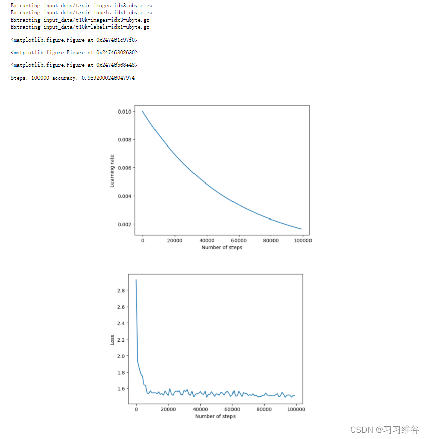
由图可知,学习率指数地下降,Loss下降地很快,测试集准确度也很快稳定下来,最终准确度约为95%,相比于之前的72%有了很大的提升。
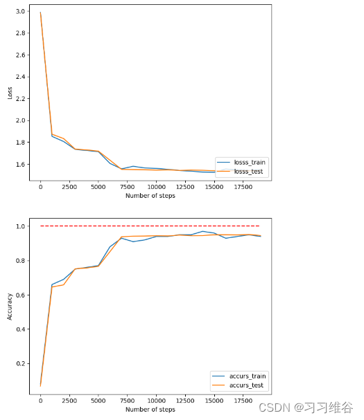
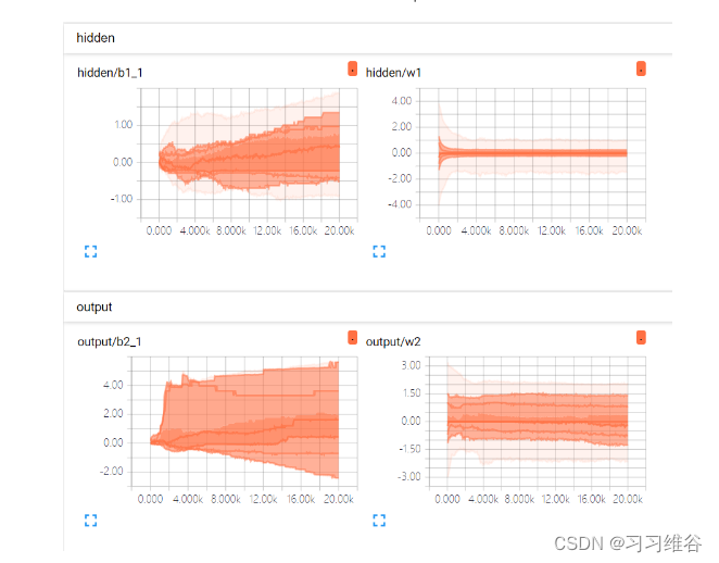
我们还可以探究每一层网络的weight、bias与迭代次数的关系
import tensorflow as tf
from tensorflow.examples.tutorials.mnist import input_data
import matplotlib.pyplot as plt

# move warning
import os

os.environ['TF_CPP_MIN_LOG_LEVEL'] = '2'
old_v = tf.logging.get_verbosity()
tf.logging.set_verbosity(tf.logging.ERROR)

# neural network parameters
INPUT_NODE = 784
LAYER1_NODE = 15
OUTPUT_NODE = 10

# exponential attenuation learning rate
LEARNING_RATE_BASE = 0.01
LEARNING_RATE_DECAY = 0.99

# regularization coefficient
LAMDA = 0.0001

# training parameters
BATCH_SIZE = 100
TRAINING_STEPS = 20000

# initialize weights and add regularization
def get_weight(weight_name, shape, lamda):
    weights = tf.Variable(tf.random_normal(shape=shape), dtype=tf.float32)
    tf.summary.histogram(weight_name, weights)
    tf.add_to_collection("losses", tf.contrib.layers.l2_regularizer(lamda)(weights))
    return weights


# read data
mnist = input_data.read_data_sets('MNIST_data/', one_hot=True)

# create model
# input layer
x = tf.placeholder(tf.float32, [None, INPUT_NODE])  # input images
y_ = tf.placeholder(tf.float32, [None, OUTPUT_NODE])  # input labels

# hidden layer
with tf.name_scope('hidden'):
    w1 = get_weight('w1', [INPUT_NODE, LAYER1_NODE], LAMDA)
    b1 = tf.Variable(tf.constant(0.1, shape=[LAYER1_NODE],name='b1'))
    tf.summary.histogram('/b1', b1)
    y1 = tf.nn.relu(tf.matmul(x, w1) + b1)

# output layer
with tf.name_scope('output'):
    w2 = get_weight('w2', [LAYER1_NODE, OUTPUT_NODE], LAMDA)
    b2 = tf.Variable(tf.constant(0.1, shape=[OUTPUT_NODE],name='b2'))
    tf.summary.histogram('/b2', b2)
    y2 = tf.nn.softmax(tf.matmul(y1, w2) + b2)

# loss function
cross_entropy = tf.reduce_mean(tf.nn.softmax_cross_entropy_with_logits(labels=y_, logits=y2))
tf.add_to_collection('losses', cross_entropy)
loss = tf.add_n(tf.get_collection('losses'))

# optimization algorithm
global_step = tf.Variable(0, trainable=False)
learning_rate = tf.train.exponential_decay(LEARNING_RATE_BASE, global_step, mnist.train.num_examples / BATCH_SIZE, LEARNING_RATE_DECAY,staircase=True)
train_step = tf.train.AdamOptimizer(learning_rate=learning_rate).minimize(loss, global_step=global_step)

# new session
sess = tf.Session()
merged = tf.summary.merge_all()
# save the logs
writer = tf.summary.FileWriter("logs/", sess.graph)
sess.run(tf.global_variables_initializer())

# train
losss_train = []
losss_test = []
accurs_train = []
accurs_test = []
steps = []
rates = []

correct_prediction = tf.equal(tf.argmax(y_, 1), tf.argmax(y2, 1))
accuracy = tf.reduce_mean(tf.cast(correct_prediction, tf.float32))
for i in range(TRAINING_STEPS):
    batch_xs, batch_ys = mnist.train.next_batch(BATCH_SIZE)
    accuracy_train, _, now_loss, step, now_learn_rate,merge= sess.run([accuracy, train_step, loss, global_step, learning_rate,merged],
                                                 feed_dict={x: batch_xs, y_: batch_ys})
    writer.add_summary(merge, i)

    if i % 1000 == 0:
        accur_test,loss_test = sess.run([accuracy,loss], feed_dict={x: mnist.test.images, y_: mnist.test.labels})
        accurs_test.append(accur_test)
        losss_test.append(loss_test)

        accurs_train.append(accuracy_train)
        losss_train.append(now_loss)

        steps.append(step)
        rates.append(now_learn_rate)


# learning rate
plt.figure()
plt.plot(steps, rates)
plt.xlabel('Number of steps')
plt.ylabel('Learning rate')

# loss
plt.figure()
plt.plot(steps, losss_train, label='losss_train')
plt.plot(steps, losss_test, label='losss_test')
plt.xlabel('Number of steps')
plt.ylabel('Loss')
plt.legend(loc='lower right')

# accuracy
plt.figure()
plt.plot(steps, accurs_train,label='accurs_train')
plt.plot(steps, accurs_test,label='accurs_test')
plt.hlines(1, 0, max(steps), colors='r', linestyles='dashed')
plt.xlabel('Number of steps')
plt.ylabel('Accuracy')
plt.legend(loc='lower right')
plt.show()

print('Accuracy: ', sess.run(accuracy, feed_dict={x: mnist.test.images, y_: mnist.test.labels}))
tf.logging.set_verbosity(old_v)
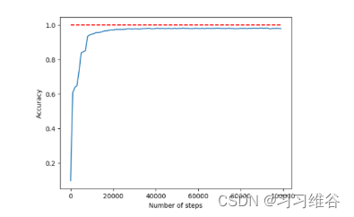
增加隐层神经元的个数
此外,通过增加隐层神经元的个数可以进一步提高神经网络的性能。例如,我们将隐层神经元由15个提高到100个,学习率初始值设为0.005,则最终准确度为98%左右,如下图所示。
import tensorflow as tf
from tensorflow.examples.tutorials.mnist import input_data
import matplotlib.pyplot as plt
import os
os.environ['TF_CPP_MIN_LOG_LEVEL'] = '2'
old_v = tf.logging.get_verbosity()
tf.logging.set_verbosity(tf.logging.ERROR)
mnist = input_data.read_data_sets('input_data/', one_hot=True)


# neural network parameters
INPUT_NODE = 784
LAYER1_NODE = 100
OUTPUT_NODE = 10

# exponential attenuation learning rate
LEARNING_RATE_BASE = 0.005
LEARNING_RATE_DECAY = 0.99

# regularization coefficient
LAMDA = 0.0001

# training parameters
BATCH_SIZE = 100
TRAINING_STEPS = 100000


# initialize weights and add regularization
def get_weight(shape, lamda):
    weights = tf.Variable(tf.random_normal(shape=shape), dtype=tf.float32)
    tf.add_to_collection("losses", tf.contrib.layers.l2_regularizer(lamda)(weights))
    return weights

# create model
# input layer
x = tf.placeholder(tf.float32, [None, INPUT_NODE])  # input images
y_ = tf.placeholder(tf.float32, [None, OUTPUT_NODE])  # input labels

# hidden layer
w1 = get_weight([INPUT_NODE, LAYER1_NODE], LAMDA)
b1 = tf.Variable(tf.constant(0.1, shape=[LAYER1_NODE]))
y1 = tf.nn.relu(tf.matmul(x, w1) + b1)

# output layer
w2 = get_weight([LAYER1_NODE, OUTPUT_NODE], LAMDA)
b2 = tf.Variable(tf.constant(0.1, shape=[OUTPUT_NODE]))
y2 = tf.nn.softmax(tf.matmul(y1, w2) + b2)

# loss function
cross_entropy = tf.reduce_mean(tf.nn.softmax_cross_entropy_with_logits(labels=y_, logits=y2))
tf.add_to_collection('losses', cross_entropy)
loss = tf.add_n(tf.get_collection('losses'))

# optimization algorithm
global_step = tf.Variable(0, trainable=False)
learning_rate = tf.train.exponential_decay(LEARNING_RATE_BASE, global_step,
                                           mnist.train.num_examples / BATCH_SIZE, LEARNING_RATE_DECAY)
train_step = tf.train.AdamOptimizer(learning_rate=learning_rate).minimize(loss, global_step=global_step)

# new session
sess = tf.Session()
sess.run(tf.global_variables_initializer())

# train
losss = []
accurs = []
steps = []
rates = []
correct_prediction = tf.equal(tf.argmax(y_, 1), tf.argmax(y2, 1))
accuracy = tf.reduce_mean(tf.cast(correct_prediction, tf.float32))
for i in range(TRAINING_STEPS):
    batch_xs, batch_ys = mnist.train.next_batch(BATCH_SIZE)
    _, now_loss, step, now_learn_rate = sess.run([train_step, loss, global_step, learning_rate],
                                                 feed_dict={x: batch_xs, y_: batch_ys})

    if i % 1000 == 0:
        accur = sess.run(accuracy, feed_dict={x: mnist.test.images, y_: mnist.test.labels})
        accurs.append(accur)
        losss.append(now_loss)
        steps.append(step)
        rates.append(now_learn_rate)

# learning rate
plt.figure()
plt.plot(steps, rates)
plt.xlabel('Number of steps')
plt.ylabel('Learning rate')

# loss
plt.figure()
plt.plot(steps, losss)
plt.xlabel('Number of steps')
plt.ylabel('Loss')

# accuracy
plt.figure()
plt.plot(steps, accurs)
plt.hlines(1, 0, max(steps), colors='r', linestyles='dashed')
plt.xlabel('Number of steps')
plt.ylabel('Accuracy')
plt.show()

tf.logging.set_verbosity(old_v)
4 卷积神经网络(CNN)
4.1 卷积操作
图像中的每一个像素点和周围的像素点是紧密联系的,但和太远的像素点就不一定有什么关联了,这就是人的视觉感受野的概念,每一个感受野只接受一小块区域的信号。这一小块区域的像素是互相关联的,每一个神经元不需要接收全部的像素点的信息,只需要接收局部的像素点作为输入,而后将这些神经元收到的局部信息综合起来就可以得到全局的信息。
图像的卷积操作就是指从图像的左上角开始,利用一个卷积模板在图像上滑动,在每一个位置将图像像素点上的像素灰度值与对应的卷积核上的数值相乘,并将所有相乘后的结果求和作为卷积核中心像素对应的卷积结果值,按照此步骤在图像的所有位置完成滑动得到卷积结果的过程。这个卷积模板在卷积神经网络中通常叫做卷积核,或滤波器,下图所示为一个图像卷积操作部分过程的示意图,图中采用33的卷积核对55大小的图片进行卷积操作。
图像卷积操作可以表示为
g
=
f
⊗
h
g = f \otimes h
g=f⊗h,其中:
g
(
i
,
j
)
=
∑
k
,
l
f
(
i
+
k
,
j
+
l
)
h
(
k
,
l
)
g(i,j) = \sum_{k,l}f(i+k,j+l)h(k,l)
g(i,j)=k,l∑f(i+k,j+l)h(k,l)
其中,f为待卷积图像的矩阵,h为卷积核函数,g为图像卷积操作的输出图像。在深度学习中,输入的图像矩阵和输出的结果矩阵都称作特征图。
4.2 池化操作
在通过卷积层获得了二维特征图之后,通常情况下特征图的尺寸仍然很大,如果直接用这些特征送给分类器进行分类,那么在计算量上将会面临很大的考验,另外也有可能出现过拟合问题,因此不方便直接用这些特征图做分类。池化操作就是为了解决这样的问题而设计的技术,它在特征图矩阵上对不同位置的特征进行聚合统计,浓缩特征。
池化操作的示意图如上图所示。常用的池化操作有两种,一种是平均池化,平均池化操作的输出是池化核对应范围内输入特征图中特征的均值;另一种是最大池化,最大池化操作的输出是池化核对应范围内输入特征图中特征的最大值。可以看出池化操作是一种特殊的图像卷积操作。
进行池化操作能显著改善卷积神经网络的效果,这主要是由于特征浓缩,特征图维度降低,卷积神经网络经常出现的过拟合现象也会相应减轻的缘故。此于,由于浓缩了一定范围内特征信息,池化操作还有增强卷积神经网络中小范围内平移不变性的作用。
4.3 卷积层
一般的卷积神经网络由多个卷积层构成,每个卷积层中通常会进行如下几个操作.
- 图像通过多个不同的卷积核的滤波,并加偏置(bias),提取出局部特征,每一个卷积核会映射出一个新的2D图像。
- 将前面的卷积核的滤波输出结果进行非线性的激活函数的处理,目前一般用ReLU函数。
- 对激活函数的结果再进行池化操作(即降采样,比如22的图片降为11的图片),目前一般是使用最大池化,保留最显著的特征,并提升模型的畸变容忍能力。
注意,一个卷积层中一般有多个不同的卷积核,因为每个卷积核只能提取一种图片特征,可以增加卷积核的数量多提取一些特征。每一个卷积核对应一个滤波后映射出的新图像,同一个新图像中的每一个像素都来自完全相同的卷积核,这就是卷积核的权值共享。共享卷积核的权值参数的目的很简单,降低模型复杂度,减轻过拟合并降低计算量。
卷积层需要训练的权值数量只和卷积核的大小以及卷积核的数量有关,我们可以使用非常少的参数处理任意大小的图片。每一个卷积层提取的特征,在后面的层中都会抽象组合成更高阶的特征。
4.4 卷积神经网络
卷积神经网络和多层感知器网络的不同之处在于,卷积神经网络包含了若干个卷积层和池化层构成的特征抽取器,可以有效地减少参数数量,大大简化模型的复杂度,从而减少过拟合的风险。同时赋予了卷积神经网络对平移和轻度变形的容忍性,提高了模型的泛化能力。
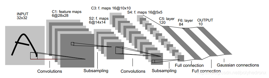
著名的LeNet5的结构如下图所示,包含了三个卷积层,一个全连接层和一个高斯连接层。一般来说,针对不同数据集、不同大小的输入图片可以根据需要合理地设计不同的卷积神经网络,来应对不同的实际问题。
用于手写数字识别问题的卷积神经网络的设计
采用两个卷积层和一个全连接层构建一个简单的卷积神经网络。
import tensorflow as tf
from tensorflow.examples.tutorials.mnist import input_data
import matplotlib.pyplot as plt

# move warning
import os
os.environ['TF_CPP_MIN_LOG_LEVEL'] = '2'
old_v = tf.logging.get_verbosity()
tf.logging.set_verbosity(tf.logging.ERROR)

mnist = input_data.read_data_sets('input_data/', one_hot=True)

# weight initialization
def weight_variable(shape):
    return tf.Variable(tf.truncated_normal(shape, stddev=0.1))


# bias initialization
def bias_variable(shape):
    return tf.Variable(tf.constant(0.1, shape=shape))


# convolution operation
def conv2d(x, W):
    return tf.nn.conv2d(x, W, strides=[1, 1, 1, 1], padding="SAME")


# pooling operation
def max_pool_2x2(x):
    return tf.nn.max_pool(x, ksize=[1, 2, 2, 1], strides=[1, 2, 2, 1], padding="SAME")


# Convolutional Neural Network
def cnn2(x):
    x_image = tf.reshape(x, [-1, 28, 28, 1])

    # Layer 1: convolutional layer
    W_conv1 = weight_variable([5, 5, 1, 32])
    b_conv1 = bias_variable([32])
    h_conv1 = tf.nn.relu(conv2d(x_image, W_conv1) + b_conv1)
    h_pool1 = max_pool_2x2(h_conv1)

    # Layer 2: convolutional layer
    W_conv2 = weight_variable([5, 5, 32, 64])
    b_conv2 = weight_variable([64])
    h_conv2 = tf.nn.relu(conv2d(h_pool1, W_conv2) + b_conv2)
    h_pool2 = max_pool_2x2(h_conv2)

    # Layer 3: full connection layer
    W_fc1 = weight_variable([7 * 7 * 64, 1024])
    b_fc1 = bias_variable([1024])
    h_pool2_flat = tf.reshape(h_pool2, [-1, 7 * 7 * 64])
    h_fc1 = tf.nn.relu(tf.matmul(h_pool2_flat, W_fc1) + b_fc1)

    # dropout layer
    keep_prob = tf.placeholder("float")
    h_fc1_drop = tf.nn.dropout(h_fc1, keep_prob)

    # output layer
    W_fc2 = weight_variable([1024, 10])
    b_fc2 = bias_variable([10])
    y_conv = tf.nn.softmax(tf.matmul(h_fc1_drop, W_fc2) + b_fc2)

    return y_conv, keep_prob

# input layer
x = tf.placeholder("float", shape=[None, 784])
y_ = tf.placeholder("float", shape=[None, 10])

# cnn
y_conv, keep_prob = cnn2(x)

# loss function & optimization algorithm
cross_entropy = tf.reduce_mean(-tf.reduce_sum(y_*tf.log(y_conv), reduction_indices=[1]))
train_step = tf.train.AdamOptimizer(1e-4).minimize(cross_entropy)

# new session
sess = tf.Session()
sess.run(tf.global_variables_initializer())

# train
losss = []
accurs = []
steps = []
correct_predict = tf.equal(tf.argmax(y_conv, 1), tf.argmax(y_, 1))
accuracy = tf.reduce_mean(tf.cast(correct_predict, "float"))
for i in range(20000):
    batch = mnist.train.next_batch(50)
    sess.run(train_step, feed_dict={x: batch[0], y_: batch[1], keep_prob: 0.5})

    if i % 100 == 0:
        loss = sess.run(cross_entropy, {x: batch[0], y_: batch[1], keep_prob: 1.0})
        accur = sess.run(accuracy, feed_dict={x: mnist.test.images, y_: mnist.test.labels, keep_prob: 1.0})
        steps.append(i)
        losss.append(loss)
        accurs.append(accur)

# plot loss
plt.figure()
plt.plot(steps, losss)
plt.xlabel('Number of steps')
plt.ylabel('Loss')

plt.figure()
plt.plot(steps, accurs)
plt.hlines(1, 0, max(steps), colors='r', linestyles='dashed')
plt.xlabel('Number of steps')
plt.ylabel('Accuracy')
plt.show()

print('Accuracy: ', sess.run(accuracy, feed_dict={x: mnist.test.images, y_: mnist.test.labels}))

tf.logging.set_verbosity(old_v)
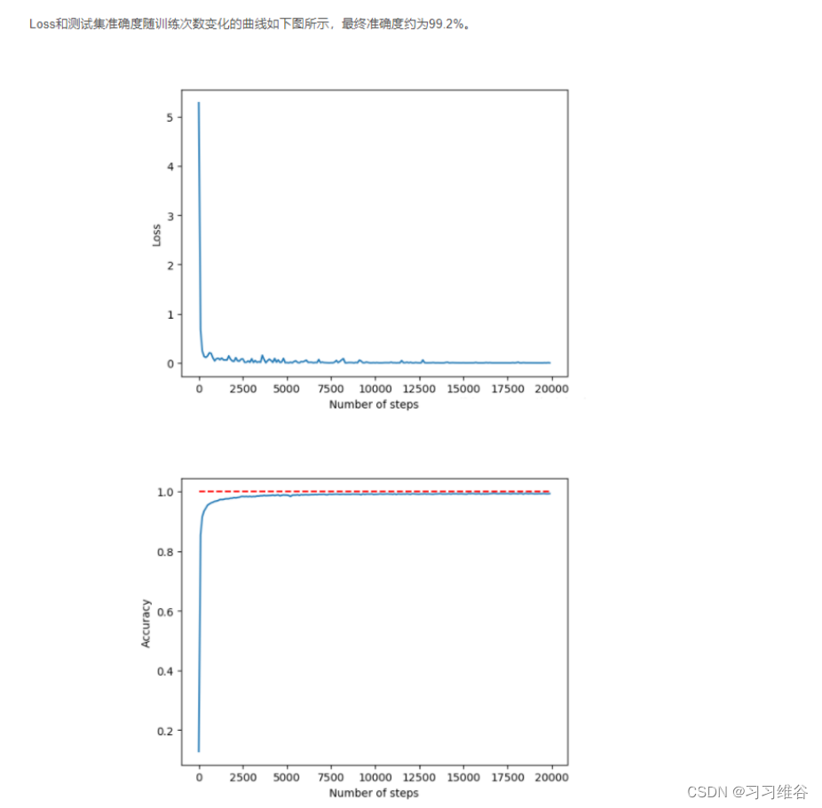
我们可以通过添加归一化层优化我们的模型
Batch Normalization(批量归一化)实现了在神经网络层的中间进行预处理的操作,即在上一层的输入归一化处理后再进入网络的下一层,这样可有效地防止“梯度弥散”,加速网络训练。
Batch Normalization具体的算法如下图所示:
每次训练时,取 batch_size 大小的样本进行训练,在BN层中,将一个神经元看作一个特征,batch_size 个样本在某个特征维度会有 batch_size 个值,然后在每个神经元
x
i
x_i
xi 维度上的进行这些样本的均值和方差,通过公式得到
x
i
^
\hat{x_i}
xi^,再通过参数
γ
\gamma
γ和
β
\beta
β进行线性映射得到每个神经元对应的输出
y
i
y_i
yi 。在BN层中,可以看出每一个神经元维度上,都会有一个参数
γ
\gamma
γ和
β
\beta
β,它们同权重
ω
\omega
ω一样可以通过训练进行优化。

在卷积神经网络中进行批量归一化时,一般对 未进行ReLu激活的 feature map进行批量归一化,输出后再作为激励层的输入,可达到调整激励函数偏导的作用。
一种做法是将 feature map 中的神经元作为特征维度,参数 γ \gamma γ和 β \beta β的数量和则等于 2 × f m a p w i d t h × f m a p l e n g t h × f m a p n u m 2×fmap_{width}×fmap_{length}×fmap_{num} 2×fmapwidth×fmaplength×fmapnum,这样做的话参数的数量会变得很多;
另一种做法是把 一个 feature map 看做一个特征维度,一个 feature map 上的神经元共享这个 feature map的 参数 γ \gamma γ和 β \beta β,参数 γ \gamma γ和 β \beta β的数量和则等于 2 × f m a p n u m 2×fmap_{num} 2×fmapnum,计算均值和方差则在batch_size个训练样本在每一个feature map维度上的均值和方差。
注: f m a p n u m fmap_{num} fmapnum指的是一个样本的feature map数量,feature map 跟神经元一样也有一定的排列顺序。
Batch Normalization 算法的训练过程和测试过程的区别:
在训练过程中,我们每次都会将 batch_size 数目大小的训练样本 放入到CNN网络中进行训练,在BN层中自然可以得到计算输出所需要的均值和方差;
而在测试过程中,我们往往只会向CNN网络中输入一个测试样本,这是在BN层计算的均值和方差会均为 0,因为只有一个样本输入,因此BN层的输入也会出现很大的问题,从而导致CNN网络输出的错误。所以在测试过程中,我们需要借助训练集中所有样本在BN层归一化时每个维度上的均值和方差,当然为了计算方便,我们可以在 batch_num 次训练过程中,将每一次在BN层归一化时每个维度上的均值和方差进行相加,最后再进行求一次均值即可。
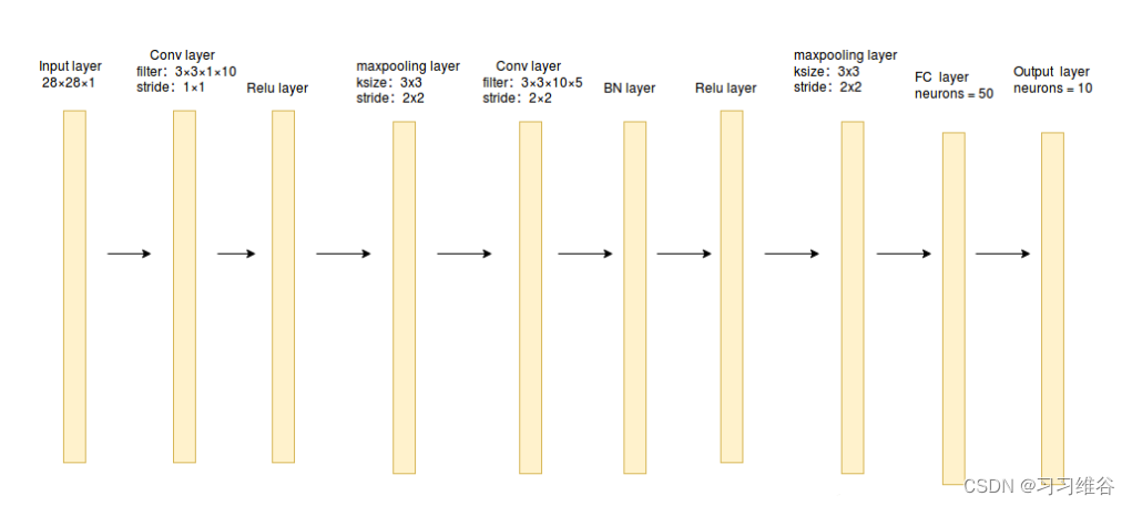
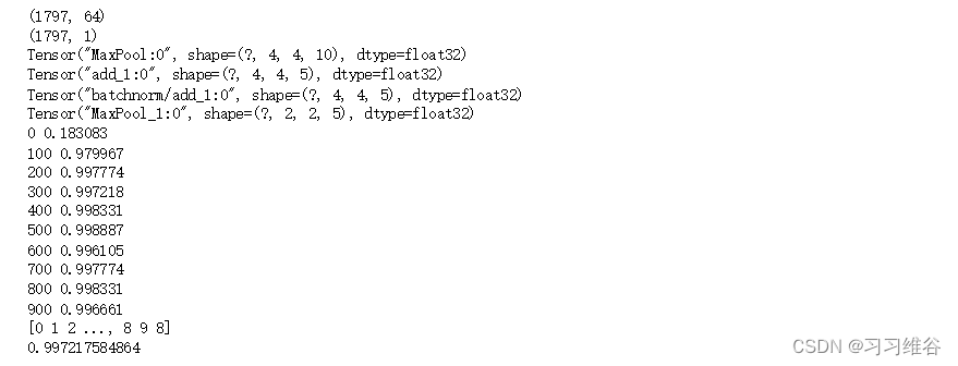
搭建的卷积神经网络结构如下图所示:
import tensorflow as tf
from sklearn.datasets import load_digits
import numpy as np
from sklearn.preprocessing import MinMaxScaler
from sklearn.preprocessing import OneHotEncoder
from sklearn.metrics import  accuracy_score

digits = load_digits()
X_data = digits.data.astype(np.float32)
Y_data = digits.target.astype(np.float32).reshape(-1,1)
print (X_data.shape)
print (Y_data.shape)

scaler = MinMaxScaler()
X_data = scaler.fit_transform(X_data)
Y = OneHotEncoder().fit_transform(Y_data).todense() #one-hot编码

# 转换为图片的格式 (batch,height,width,channels)
X = X_data.reshape(-1,8,8,1)

batch_size = 8 # 使用MBGD算法,设定batch_size为8

def generatebatch(X,Y,n_examples, batch_size):
    for batch_i in range(n_examples // batch_size):
        start = batch_i*batch_size
        end = start + batch_size
        batch_xs = X[start:end]
        batch_ys = Y[start:end]
        yield batch_xs, batch_ys # 生成每一个batch

tf.reset_default_graph()
# 输入层
tf_X = tf.placeholder(tf.float32,[None,8,8,1])
tf_Y = tf.placeholder(tf.float32,[None,10])

# 卷积层+激活层
conv_filter_w1 = tf.Variable(tf.random_normal([3, 3, 1, 10]))
conv_filter_b1 =  tf.Variable(tf.random_normal([10]))
relu_feature_maps1 = tf.nn.relu(\
                tf.nn.conv2d(tf_X, conv_filter_w1,strides=[1, 1, 1, 1], padding='SAME') + conv_filter_b1)

# 池化层
max_pool1 = tf.nn.max_pool(relu_feature_maps1,ksize=[1,3,3,1],strides=[1,2,2,1],padding='SAME')

print (max_pool1)

# 卷积层
conv_filter_w2 = tf.Variable(tf.random_normal([3, 3, 10, 5]))
conv_filter_b2 =  tf.Variable(tf.random_normal([5]))
conv_out2 = tf.nn.conv2d(relu_feature_maps1, conv_filter_w2,strides=[1, 2, 2, 1], padding='SAME') + conv_filter_b2
print(conv_out2)
# BN归一化层+激活层
batch_mean, batch_var = tf.nn.moments(conv_out2, [0, 1, 2], keep_dims=True)
shift = tf.Variable(tf.zeros([5]))
scale = tf.Variable(tf.ones([5]))
epsilon = 1e-3
BN_out = tf.nn.batch_normalization(conv_out2, batch_mean, batch_var, shift, scale, epsilon)
print(BN_out)
relu_BN_maps2 = tf.nn.relu(BN_out)

# 池化层
max_pool2 = tf.nn.max_pool(relu_BN_maps2,ksize=[1,3,3,1],strides=[1,2,2,1],padding='SAME')
print(max_pool2)

# 将特征图进行展开
max_pool2_flat = tf.reshape(max_pool2, [-1, 2*2*5])

# 全连接层
fc_w1 = tf.Variable(tf.random_normal([2*2*5,50]))
fc_b1 =  tf.Variable(tf.random_normal([50]))
fc_out1 = tf.nn.relu(tf.matmul(max_pool2_flat, fc_w1) + fc_b1)

# 输出层
out_w1 = tf.Variable(tf.random_normal([50,10]))
out_b1 = tf.Variable(tf.random_normal([10]))
pred = tf.nn.softmax(tf.matmul(fc_out1,out_w1)+out_b1)

loss = -tf.reduce_mean(tf_Y*tf.log(tf.clip_by_value(pred,1e-11,1.0)))
train_step = tf.train.AdamOptimizer(1e-3).minimize(loss)
y_pred = tf.arg_max(pred,1)
bool_pred = tf.equal(tf.arg_max(tf_Y,1),y_pred)
accuracy = tf.reduce_mean(tf.cast(bool_pred,tf.float32)) # 准确率

with tf.Session() as sess:
    sess.run(tf.global_variables_initializer())
    for epoch in range(1000): # 迭代1000个周期
        for batch_xs,batch_ys in generatebatch(X,Y,Y.shape[0],batch_size): # 每个周期进行MBGD算法
            sess.run(train_step,feed_dict={tf_X:batch_xs,tf_Y:batch_ys})
        if(epoch%100==0):
            res = sess.run(accuracy,feed_dict={tf_X:X,tf_Y:Y})
            print (epoch,res)
    res_ypred = y_pred.eval(feed_dict={tf_X:X,tf_Y:Y}).flatten() # 只能预测一批样本,不能预测一个样本
    print (res_ypred)

print(accuracy_score(Y_data,res_ypred.reshape(-1,1)))


 1387
1387


 被折叠的 条评论
为什么被折叠?
被折叠的 条评论
为什么被折叠?
 到【灌水乐园】发言


