数据分析之numpy(基本使用详细)

一,什么是numpy

官方文档:https://numpy.org/doc/stable/user/quickstart.html

NumPy系统是Python的一种开源的数值计算扩展，这种工具可用来存储和处理大型矩阵，比Python自身的嵌套列表（nested list structure)结构要高效的多（该结构也可以用来表示矩阵（matrix））。

1,Numpy相关介绍：

一个用python实现的科学计算包括：

1、一个强大的N维数组对象Array；

2、比较成熟的（广播）函数库；

3、用于整合C/C++和Fortran代码的工具包；

4、实用的线性代数、傅里叶变换和随机数生成函数。numpy和稀疏矩阵运算包scipy配合使用更加方便。

2,NumPy包的核心是ndarray对象。

这封装了同构数据类型的n维数组，许多操作在编译代码中执行以提高性能。NumPy数组和标准Python序列之间有几个重要的区别：

•NumPy数组在创建时具有固定大小，与Python列表（可以动态增长）不同。更改ndarray的大小将创建一个新数组并删除原始数组。

•NumPy数组中的元素都需要具有相同的数据类型，因此在内存中的大小相同。例外：可以有（Python，包括NumPy）对象的数组，从而允许不同大小的元素的数组。

•NumPy数组有助于对大量数据进行高级数学和其他类型的操作。通常，与使用Python的内置序列相比，这些操作的执行效率更高，代码更少。

NumPy - Ndarray 对象
NumPy 中定义的最重要的对象是称为 ndarray 的 N 维数组类型。 它描述相同类型的元素集合。 可以使用基于零的索引访问集合中的项目。

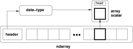
ndarray中的每个元素在内存中使用相同大小的块。 ndarray中的每个元素是数据类型对象的对象（称为 dtype）。

从ndarray对象提取的任何元素（通过切片）由一个数组标量类型的 Python 对象表示。 下图显示了ndarray，数据类型对象（dtype）和数组标量类型之间的关系。

二,基本使用

pip install numpay

1,创建数组对象(numpy.ndarray)

import numpy as np
#import numpy as np

np.array(12)
#array(12)

np.array([12])
#array([12])

np.array(range(12))
#array([ 0,  1,  2,  3,  4,  5,  6,  7,  8,  9, 10, 11])

type(np.array(range(12)))
#numpy.ndarray

array原型和相关说明,他接受一个对象或者序列化的数组,dtype指数组类型

1.object 任何暴露数组接口方法的对象都会返回一个数组或任何（嵌套）序列。
2. dtype 数组的所需数据类型，可选。
3. copy 可选，默认为true，对象是否被复制。
4. order C（按行）、F（按列）或A（任意，默认）。
5. subok 默认情况下，返回的数组被强制为基类数组。 如果为true，则返回子类。
6. ndmin 指定返回数组的最小维数。

def array(object, dtype=None, copy=True, order='K', subok=False, ndmin=0)
	Create an array.
	
	Parameters
	object : array_like
	
	    An array, any object exposing the array interface, an object whose  
	    __array__ method returns an array, or any (nested) sequence.  
	dtype : data-type, optional
	
	    The desired data-type for the array.  If not given, then the type will  
	    be determined as the minimum type required to hold the objects in the  
	    sequence.  
	copy : bool, optional
	
	    If true (default), then the object is copied.  Otherwise, a copy will  
	    only be made if __array__ returns a copy, if obj is a nested sequence,  
	    or if a copy is needed to satisfy any of the other requirements  
	    (`dtype`, `order`, etc.).  
	order : {'K', 'A', 'C', 'F'}, optional
	
	    Specify the memory layout of the array. If object is not an array, the  
	    newly created array will be in C order (row major) unless 'F' is  
	    specified, in which case it will be in Fortran order (column major).  
	    If object is an array the following holds.  
	
	    ===== ========= ===================================================  
	    order  no copy                     copy=True  
	    ===== ========= ===================================================  
	    'K'   unchanged F & C order preserved, otherwise most similar order  
	    'A'   unchanged F order if input is F and not C, otherwise C order  
	    'C'   C order   C order  
	    'F'   F order   F order  
	    ===== ========= ===================================================  
	
	    When `copy=False` and a copy is made for other reasons, the result is  
	    the same as if `copy=True`, with some exceptions for `A`, see the  
	    Notes section. The default order is 'K'.  
	subok : bool, optional
	
	    If True, then sub-classes will be passed-through, otherwise  
	    the returned array will be forced to be a base-class array (default).  
	ndmin : int, optional
	
	    Specifies the minimum number of dimensions that the resulting  
	    array should have.  Ones will be pre-pended to the shape as  
	    needed to meet this requirement.  
	Returns
	out : ndarray
	
	    An array object satisfying the specified requirements.

原谅我也看不出来啥,哈哈(学生小白一枚),分享欲太重了

ndarray的方法

Ndarray.ndim 数组的轴数(尺寸)。

Ndarray.shape
数组的尺寸。这是一个整数元组，指示每个维度中数组的大小。的矩阵n行和m纵队，shape将是(n,m)。的长度shape元组是轴的数目，ndim.

Ndarray.size 数组的元素总数。元素的乘积。shape.

Ndarray.dtype
描述数组中元素类型的对象。可以使用标准Python类型创建或指定dtype。此外，NumPy还提供自己的类型。Numpy.int
32、numpy.int 16和numpy.Float 64是一些例子。

Ndarray.itemsize
数组中每个元素的大小(以字节为单位)。例如，类型的元素数组float64有itemsize8(=64/8)，而类型之一complex32有itemsize4(=32/8)。它相当于ndarray.dtype.itemsize.

Ndarray.data 包含数组实际元素的缓冲区。通常，我们不需要使用这个属性，因为我们将使用索引工具访问数组中的元素。

2,创建数组

np.arange(10)
#array([0, 1, 2, 3, 4, 5, 6, 7, 8, 9])
list(range(10))
#[0, 1, 2, 3, 4, 5, 6, 7, 8, 9]

def arange(start=None, stop, step=None, , dtype=None)
	Return evenly spaced values within a given interval.

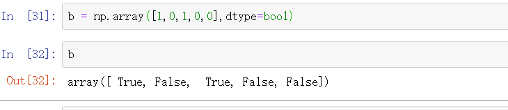
以指定类型创建

b = np.array([1,0,1,0,0],dtype=bool)
#array([ True, False,  True, False, False])

修改数据类型

b.astype('int32')
array([1, 0, 1, 0, 0])

保留三位小鼠

b = random.random()

b
#0.650550873542433

np.round(b,3)
#0.650

根据形状构建数组

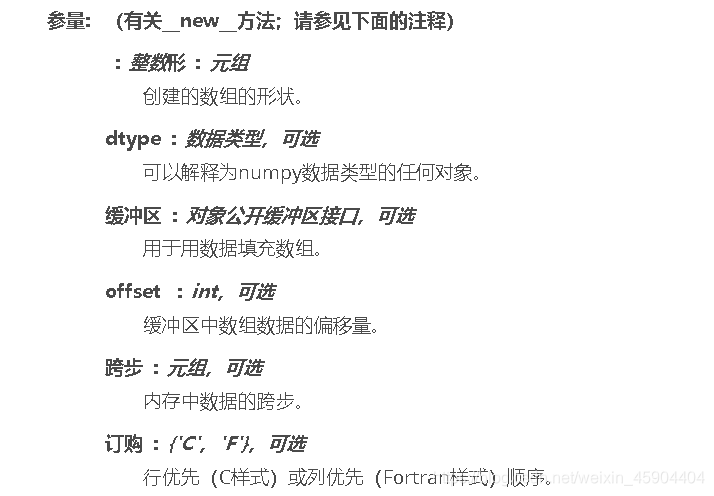
类numpy.ndarray（shape，dtype = float，buffer = None，offset = 0，strides = None，order = None ）[资源]
数组对象表示固定大小项目的多维同构数组。关联的数据类型对象描述了数组中每个元素的格式（其字节顺序，它在内存中占用多少字节，它是整数，浮点数还是其他，等等）

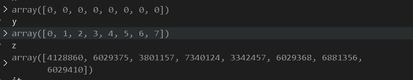
>>> np.ndarray((2,2,2),dtype='int') 
array([[[4128860, 6029375],
        [3801157, 7340124]],

       [[3342457, 6029368],
        [4980804, 7536716]]])
>>> np.ndarray((2,2,2),dtype='int',buffer=b) 
array([[[2, 3],
        [4, 5]],

       [[6, 3],
        [4, 5]]])
>>> b
array([[2, 3, 4, 5, 6],
       [3, 4, 5, 6, 7],
       [8, 9, 0, 1, 2]])

构建初始数组

numpy.zeros（shape，dtype = float，order =‘C’，*，like = None ）

>>> np.zeros((2,2))                  
array([[0., 0.],
       [0., 0.]])
>>>

3,数组类型

NumPy 支持比 Python 更多种类的数值类型。 下表显示了 NumPy 中定义的不同标量数据类型。
数组类型

>>>np.arange(10).dtype 
dtype('int32')
>>> dt = np.dtype('>i4')
>>> dt.byteorder
'>'
>>> dt.itemsize
4
>>> dt.name
'int32'

dtype(obj[, align, copy]) 创建数据类型对象。 可以转换为数据类型对象的内容如下：

1. bool_ 存储为一个字节的布尔值（真或假）
2. int_ 默认整数，相当于 C 的long，通常为int32或int64
3. intc 相当于 C 的int，通常为int32或int64
4. intp 用于索引的整数，相当于 C 的size_t，通常为int32或int64
5. int8 字节（-128 ~ 127）
6. int16 16 位整数（-32768 ~ 32767）
7. int32 32 位整数（-2147483648 ~ 2147483647）
8. int64 64 位整数（-9223372036854775808 ~ 9223372036854775807）
9. uint8 8 位无符号整数（0 ~ 255）
10. uint16 16 位无符号整数（0 ~ 65535）
11. uint32 32 位无符号整数（0 ~ 4294967295）
12. uint64 64 位无符号整数（0 ~ 18446744073709551615）
13. float_ float64的简写
14. float16 半精度浮点：符号位，5 位指数，10 位尾数
15. float32 单精度浮点：符号位，8 位指数，23 位尾数
16. float64 双精度浮点：符号位，11 位指数，52 位尾数
17. complex_ complex128的简写
18. complex64 复数，由两个 32 位浮点表示（实部和虚部）
19. complex128 复数，由两个 64 位浮点表示（实部和虚部）

dtype
[(field_name, field_dtype, field_shape), …]
第一个元素 field_name 是字段名称(如果这是 ‘’ ，则分配标准字段名称 ‘f#’)。字段名称也可以是字符串的2元组，其中第一个字符串是“title”（可以是任何字符串或Unicode字符串）或字段的元数据，该字段可以是任何对象，
第二个元素 field_dtype 可以是任何可以解释为数据类型的元素。
第三个参数是此类型所需的形状。如果Shape参数为1，则数据类型对象等同于固定dtype。 如果 shape 是一个元组，那么新的dtype定义了给定形状的子数组。

In [65]: a= np.array([('a', (8.0, 7.0,9.0)),('s',(1.0,2,8))], dtype=[('name', np.unicode_,10), ('num', np.float64,3)])
In [67]: a['name']
Out[67]: array(['a', 's'], dtype='<U10')

In [68]: a['num']
Out[68]: 
array([[8., 7., 9.],
       [1., 2., 8.]])`

数据类型的一些方法

dtype.type 用于实例化此数据类型的标量的类型对象。
dtype.kind 识别一般数据类型的字符码( “biufcmMOSUV” 之一)。
dtype.char 21种不同内置类型中的每一种都有唯一的字符码。
dtype.num 21种不同内置类型中每种类型的唯一编号。
dtype.str 此数据类型对象的数组协议类型字符串。
数据的大小依次由以下内容描述：

方法 描述
dtype.name 此数据类型的位宽名称。
dtype.itemsize 此数据类型对象的元素大小。
此数据的字符顺序：

方法 描述
dtype.byteorder 指示此数据类型对象的字节顺序的字符。
有关结构化数据类型中的子数据类型的信息：

方法 描述
dtype.fields 为此数据类型定义的命名字段的字典，或 None。
dtype.names 字段名称的有序列表，如果没有字段，则为 None。
对于描述子数组的数据类型：

方法 描述
dtype.subdtype 元组 (item_dtype，shape)。如果此dtype描述子数组，则无其他。
dtype.shape 如果此数据类型描述子数组，则为子数组的Shape元组，否则为 ()。
提供附加信息的属性：

方法 描述
dtype.hasobject 指示此数据类型在任何字段或子数据类型中是否包含任何引用计数对象的布尔值。
dtype.flags 描述如何解释此数据类型的位标志。
dtype.isbuiltin 指示此数据类型如何与内置数据类型相关的整数。
dtype.isnative 指示此dtype的字节顺序是否为平台固有的布尔值。
dtype.descr array_interface 数据类型说明。
dtype.alignment 根据编译器，此数据类型所需的对齐(字节)。
dtype.base 返回子数组的基本元素的dtype，而不考虑其尺寸或形状。
#方法
数据类型具有以下更改字节顺序的方法：

方法 描述
dtype.newbyteorder([new_order]) 返回具有不同字节顺序的新dtype。
以下方法实现腌制（pickle）协议：

方法 描述
dtype.reduce() 帮助腌制（pickle）
dtype.setstate()

4,数组形状

>>> b
array([array([0, 1, 2, 3, 4, 5, 6, 7, 8, 9]),
       list([array([0, 1, 2, 3, 4, 5, 6, 7, 8, 9])])], dtype=object)
>>> b.shape
(2,)
>>> d
array([list([1, 2, 2, 2]), list([2, 234, [5, 3], 3]), 23, list([1, 3])],dtype=object)
>>> d.shape
(4,)
>>>> b = np.array([[1,2,3,4,5],[1,2,3,4,5],[1,23,4,5,6]])
>>>> b.shape
(3, 5)  #代表3行,每行5个

结果有点出乎意料
修改行状

>>> b.reshape(1,15) 
array([[ 1,  2,  3,  4,  5,  1,  2,  3,  4,  5,  1, 23,  4,  5,  6]])
>>> b.reshape(5,3)
array([[ 1,  2,  3],
       [ 4,  5,  1],
       [ 2,  3,  4],
       [ 5,  1, 23],
       [ 4,  5,  6]])

5.数组的计算

-+*%@<>/

>>> a = np.array( [20,30,40,50] )
>>> a-5
array([15, 25, 35, 45])
>>> b = np.arange( 4 )
>>> b
array([0, 1, 2, 3])
>>> c = a-b
>>> c
array([20, 29, 38, 47])
>>> b**2
array([0, 1, 4, 9])
>>> a<35
array([ True,  True, False, False])
>>> a+b
array([20, 31, 42, 53])
>>> a@b
260
>>> a%b
<stdin>:1: RuntimeWarning: divide by zero encountered in remainder
array([0, 0, 0, 2], dtype=int32)
>>> a*b
array([  0,  30,  80, 150])
>>> a-b
array([20, 29, 38, 47])
>>> a-a
array([0, 0, 0, 0])
>>> a-a-a
array([-20, -30, -40, -50])

相同维度计算

>>>	d =np.array([1,2,3,4,5])
>>> b
array([[ 1,  2,  3,  4,  5],
       [ 1,  2,  3,  4,  5],
       [ 1, 23,  4,  5,  6]])
>>> d*b
array([[ 1,  4,  9, 16, 25],
       [ 1,  4,  9, 16, 25],
       [ 1, 46, 12, 20, 30]])
>>> a = np.array([[1,2,3,4,5],[1,2,3,4,5]]) 
>>> a
array([[1, 2, 3, 4, 5],
       [1, 2, 3, 4, 5]])
>>> b = np.array([[2,],[3,]])
>>> b
array([[2],
       [3]])
>>> a*b
array([[ 2,  4,  6,  8, 10],
       [ 3,  6,  9, 12, 15]])

不同维度,形状不同不能计算

>>> a = np.array([2,3,4])
>>> a*b
Traceback (most recent call last):
  File "<stdin>", line 1, in <module>
ValueError: operands could not be broadcast together with shapes (3,) (3,5)

我们来看下三维和二维之间的计算

>>> a = np.array([[[1,2,3,4,5],[21,22,23,24,25],[31,32,33,34,35]],[[111,222,333,444,555],[666,777,888,999,1000],[122,222,233,244,255]]) 
  File "<stdin>", line 1
    a = np.array([[[1,2,3,4,5],[21,22,23,24,25],[31,32,33,34,35]],[[111,222,333,444,555],[666,777,888,999,1000],[122,222,233,244,255]])  
                                                                                                                                      ^  
SyntaxError: closing parenthesis ')' does not match opening parenthesis '['
>>> a = np.array([[[1,2,3,4,5],[21,22,23,24,25],[31,32,33,34,35]],[[111,222,333,444,555],[666,777,888,999,1000],[122,222,233,244,255]]]) 
>>> a.shape
(2, 3, 5)
>>> a
array([[[   1,    2,    3,    4,    5],
        [  21,   22,   23,   24,   25],
        [  31,   32,   33,   34,   35]],

       [[ 111,  222,  333,  444,  555],
        [ 666,  777,  888,  999, 1000],
        [ 122,  222,  233,  244,  255]]])
>>> b = np.array([[2,3,4,5,6],[3,4,5,6,7]])
>>> b
array([[2, 3, 4, 5, 6],
       [3, 4, 5, 6, 7]])
>>> b.shape
(2, 5)
>>> a-b
Traceback (most recent call last):
  File "<stdin>", line 1, in <module>
ValueError: operands could not be broadcast together with shapes (2,3,5) (2,5)
>>> b = np.array([[2,3,4,5,6],[3,4,5,6,7],[8,9,0,1,2]]) 
>>> b.shape
(3, 5)
>>> a-b
array([[[ -1,  -1,  -1,  -1,  -1],
        [ 18,  18,  18,  18,  18],
        [ 23,  23,  33,  33,  33]],

       [[109, 219, 329, 439, 549],
        [663, 773, 883, 993, 993],
        [114, 213, 233, 243, 253]]])
>>> a*b
array([[[   2,    6,   12,   20,   30],
        [  63,   88,  115,  144,  175],
        [ 248,  288,    0,   34,   70]],

       [[ 222,  666, 1332, 2220, 3330],
        [1998, 3108, 4440, 5994, 7000],
        [ 976, 1998,    0,  244,  510]]])

总结:广播的原则

广播的原则：如果两个数组的后缘维度（trailing dimension，即从末尾开始算起的维度）的轴长度相符，或其中的一方的长度为1，则认为它们是广播兼容的。广播会在缺失和（或）长度为1的维度上进行。

6,常用函数

numpy中有很多函数,三角函数,位运算,比较浮动,更多请看官方文档

数学运算

add(x1, x2, /[, out, where, cast, order, …]) 按元素添加参数。
subtract(x1, x2, /[, out, where, cast, …]) 从元素方面减去参数。
multiply(x1, x2, /[, out, where, cast, …]) 在元素方面乘以论证。
divide(x1, x2, /[, out, where, cast, …]) 以元素方式返回输入的真正除法。
logaddexp(x1, x2, /[, out, where, cast, …]) 输入的取幂之和的对数。
logaddexp2(x1, x2, /[, out, where, cast, …]) base-2中输入的取幂之和的对数。
true_divide(x1, x2, /[, out, where, …]) 以元素方式返回输入的真正除法。
floor_divide(x1, x2, /[, out, where, …]) 返回小于或等于输入除法的最大整数。
negative(x, /[, out, where, cast, order, …]) 数字否定, 元素方面。
positive(x, /[, out, where, cast, order, …]) 数字正面, 元素方面。
power(x1, x2, /[, out, where, cast, …]) 第一个数组元素从第二个数组提升到幂, 逐个元素。
remainder(x1, x2, /[, out, where, cast, …]) 返回除法元素的余数。
mod(x1, x2, /[, out, where, cast, order, …]) 返回除法元素的余数。
fmod(x1, x2, /[, out, where, cast, …]) 返回除法的元素余数。
divmod(x1, x2 [, out1, out2], /[[, out, …]) 同时返回逐元素的商和余数。
absolute(x, /[, out, where, cast, order, …]) 逐个元素地计算绝对值。
fabs(x, /[, out, where, cast, order, …]) 以元素方式计算绝对值。
rint(x, /[, out, where, cast, order, …]) 将数组的元素舍入为最接近的整数。
sign(x, /[, out, where, cast, order, …]) 返回数字符号的元素指示。
heaviside(x1, x2, /[, out, where, cast, …]) 计算Heaviside阶跃函数。
conj(x, /[, out, where, cast, order, …]) 以元素方式返回复共轭。
conjugate(x, /[, out, where, cast, …]) 以元素方式返回复共轭。
exp(x, /[, out, where, cast, order, …]) 计算输入数组中所有元素的指数。
exp2(x, /[, out, where, cast, order, …]) 计算输入数组中所有 p 的 2**p。
log(x, /[, out, where, cast, order, …]) 自然对数, 元素方面。
log2(x, /[, out, where, cast, order, …]) x的基数为2的对数。
log10(x, /[, out, where, cast, order, …]) 以元素方式返回输入数组的基数10对数。
expm1(x, /[, out, where, cast, order, …]) 计算数组中的所有元素。exp(x) - 1
log1p(x, /[, out, where, cast, order, …]) 返回一个加上输入数组的自然对数, 逐个元素。
sqrt(x, /[, out, where, cast, order, …]) 以元素方式返回数组的非负平方根。
square(x, /[, out, where, cast, order, …]) 返回输入的元素方块。
cbrt(x, /[, out, where, cast, order, …]) 以元素方式返回数组的立方根。
reciprocal(x, /[, out, where, cast, …]) 以元素方式返回参数的倒数。
gcd(x1, x2, /[, out, where, cast, order, …]) 返回 | x1 | 和的最大公约数 | x2 | 。
lcm(x1, x2, /[, out, where, cast, order, …]) 返回 | x1 | 和的最小公倍数 | x2 | 。

>>> B = np.arange(3)
>>> B
array([0, 1, 2])
>>> np.exp(B)
array([1.        , 2.71828183, 7.3890561 ])
>>> np.sqrt(B)
array([0.        , 1.        , 1.41421356])
>>> C = np.array([2., -1., 4.])
>>> np.add(B, C)
array([2., 0., 6.])

浮动

isfinite(x, /[, out, where, cast, order, …]) 测试元素的有限性(不是无穷大或不是数字)。
isinf(x, /[, out, where, cast, order, …]) 正面或负面无穷大的元素测试。
isnan(x, /[, out, where, cast, order, …]) 测试NaN的元素, 并将结果作为布尔数组返回。
isnat(x, /[, out, where, cast, order, …]) 为NaT(不是时间)测试元素, 并将结果作为布尔数组返回。
fabs(x, /[, out, where, cast, order, …]) 以元素方式计算绝对值。
signbit(x, /[, out, where, cast, order, …]) 返回元素为True设置signbit(小于零)。

其他方法

>>>a
array([[ 0,  1,  2,  3,  4],
       [ 5,  6,  7,  8,  9],
       [10, 11, 12, 13, 14]])
>>>a.shape
(3, 5)
>>>a.ndim
2
>>>a.dtype.name
'int64'
>>>a.itemsize
8
>>>a.size
15
>>>type(a)
<class 'numpy.ndarray'>
>>>b = np.array([6, 7, 8])
>>> [i for i in b.flat]  #b.flat返回一个迭代器
[6, 7, 8]
>>>type(b)
<class 'numpy.ndarray'>
>>>[x for x in a.flat] 

所有方法

三,读取文件

由于csv便于展示,读取和写入,所以很多地方也是用csv的格式存储和传输中小型的数据,
为了方便教学,我们会经常操作csv格式的文件,但是操作数据库中的数据也是很容易的实现的

np.loadtxt(fname,dtype=np.float,delimiter=None,skiprows=0,
usecols=None,unpack=False)

参数 解释
frame 文件、字符串或产生器,可以是.gz或bz2压缩文件
dtype 数据类型,可选,CSV的字符串以什么数据类型读入数组中,默认np.float
delimiter 分隔字符串,默认是任何空格,改为逗号
skiprows 跳过前x行,一般跳过第一行表头
usecols 读取指定的列,索引,元组类型
unpack 如果True,读入属性将分别写入不同数组变量,
False 读入数据只写入一个数组变量,默认False

import numpy as np
from matplotlib import  pyplot as plt

uk_file_path = "./GB_video_data_numbers.csv"

# t1 = np.loadtxt(us_file_path,delimiter=",",dtype="int",unpack=True)
t_uk =  np.loadtxt(uk_file_path,delimiter=",",dtype="int") 
#选择喜欢书比50万小的数据
t_uk = t_uk[t_uk[:,1]<=500000]

t_uk_comment = t_uk[:,-1]
t_uk_like = t_uk[:,1]


plt.figure(figsize=(20,8),dpi=80)
plt.scatter(t_uk_like,t_uk_comment) #绘制散点图

plt.show()

不懂matplotlib 的请看上一篇

四,索引、切片和迭代

NumPy切片创建视图而不是复制

视图 在不接触基础数据的情况下，NumPy可以使一个数组看起来改变其数据类型和形状。

这样创建的数组就是一个视图，而NumPy经常利用使用视图而不是制作一个新数组来提高性能。

潜在的缺点是，写入视图也可以更改原始视图。如果这是一个问题，则NumPy需要创建一个物理上不同的数组–一个copy

>>> x = np.array([0, 1, 2, 3, 4, 5, 6, 7, 8, 9])
>>> x[1:7:2]
array([1, 3, 5])

[start:stop:step]

>>> c = np.arange(12) 
>>> c[::-1] 
array([11, 10,  9,  8,  7,  6,  5,  4,  3,  2,  1,  0])
>>> c[-3:3:-1] 
array([9, 8, 7, 6, 5, 4])
>>> c[-3:3]    
array([], dtype=int32)
>>> c
array([ 0,  1,  2,  3,  4,  5,  6,  7,  8,  9, 10, 11])
>>> c[3:-3] 
array([3, 4, 5, 6, 7, 8])
>>> c[3:-3:-1] 
array([], dtype=int32)
>>> c[3:-3:1]  
array([3, 4, 5, 6, 7, 8])

查看其他维度

Ellipsis扩展:为选择元组索引所有维度所需的对象数。在大多数情况下，这意味着扩展选择元组的长度是x.ndim。可能只存在一个省略号。

>>> c[...,0] 
array(0)
>>> c
array([ 0,  1,  2,  3,  4,  5,  6,  7,  8,  9, 10, 11])
>>> a
array([[[   1,    2,    3,    4,    5],
        [  21,   22,   23,   24,   25],
        [  31,   32,   33,   34,   35]],

       [[ 111,  222,  333,  444,  555],
        [ 666,  777,  888,  999, 1000],
        [ 122,  222,  233,  244,  255]]])
>>> a[...,0] 
array([[  1,  21,  31],
       [111, 666, 122]])
>>> a[...,...,0] 
Traceback (most recent call last):
  File "<stdin>", line 1, in <module>
IndexError: an index can only have a single ellipsis ('...')

增加维度

该newaxis对象可用于所有切片操作，以创建长度为1的轴。newaxis是’None’的别名，'None’可以用来代替相同的结果。

>>> c
array([ 0,  1,  2,  3,  4,  5,  6,  7,  8,  9, 10, 11])
>>> c[:np.newaxis] 
array([ 0,  1,  2,  3,  4,  5,  6,  7,  8,  9, 10, 11])
>>> c[:,np.newaxis].shape 
(12, 1)
>>> c[:,np.newaxis]      
array([[ 0],
       [ 1],
       [ 2],
       [ 3],
       [ 4],
       [ 5],
       [ 6],
       [ 7],
       [ 8],
       [ 9],
       [10],
       [11]])

高级索引

高级索引始终作为 一个 整体进行 广播 和迭代：

result[i_1, …, i_M] == x[ind_1[i_1, …, i_M], ind_2[i_1, …, i_M],
…, ind_N[i_1, …, i_M]]

>>> a[:,[1,2]]  
array([[[  21,   22,   23,   24,   25],
        [  31,   32,   33,   34,   35]],

       [[ 666,  777,  888,  999, 1000],
        [ 122,  222,  233,  244,  255]]])
>>> a[[0,1],[1,2]]   #行索引0,1 列索引1,2
array([[ 21,  22,  23,  24,  25],
       [122, 222, 233, 244, 255]])
>>> a[0][1:] 
array([[21, 22, 23, 24, 25],
       [31, 32, 33, 34, 35]])

数组作为索引

>>> x = array([[ 0,  1,  2],
...            [ 3,  4,  5],
...            [ 6,  7,  8],
...            [ 9, 10, 11]])
>>> rows = np.array([[0, 0],
...                  [3, 3]], dtype=np.intp)
>>> columns = np.array([[0, 2],
...                     [0, 2]], dtype=np.intp)
>>> x[rows, columns]
array([[ 0,  2],
       [ 9, 11]])
>>> x[np.ix_(rows, columns)]
array([[ 0,  2],
       [ 9, 11]])

高级索引加基本索引

>>> a[1:,2:] 
array([[[122, 222, 233, 244, 255]]])

运算符索引

>>> d[d>2] 
array([ 3,  4,  5,  6,  7,  8,  9, 10, 11])
>>> d
array([ 0,  1,  2,  3,  4,  5,  6,  7,  8,  9, 10, 11])
>>> a[a>1] 
array([   2,    3,    4,    5,   21,   22,   23,   24,   25,   31,   32,
         33,   34,   35,  111,  222,  333,  444,  555,  666,  777,  888,
        999, 1000,  122,  222,  233,  244,  255])
>>> a
array([[[   1,    2,    3,    4,    5],
        [  21,   22,   23,   24,   25],
        [  31,   32,   33,   34,   35]],

       [[ 111,  222,  333,  444,  555],
        [ 666,  777,  888,  999, 1000],
        [ 122,  222,  233,  244,  255]]])

布尔值索引

>>> rows = (a>=d.sum())
>>> rows
array([[[False, False, False, False, False],
        [False, False, False, False, False],
        [False, False, False, False, False]],

       [[ True,  True,  True,  True,  True],
        [ True,  True,  True,  True,  True],
        [ True,  True,  True,  True,  True]]])

字段类型访问索引

如果ndarray对象是结构化数组 ，则可以通过使用字符串索引数组来访问数组的字段，类似于字典。

>>> x = np.zeros((2,2), dtype=[('a', np.int32), ('b', np.float64, (3,3))])
>>> x['a'].shape
(2, 2)
>>> x['a'].dtype
dtype('int32')
>>> x['b'].shape
(2, 2, 3, 3)
>>> x['b'].dtype
dtype('float64')

裁剪

`>>> a.clip(10) 
array([[[10, 10, 10, 10],
        [10, 10, 10, 10],
        [10, 10, 10, 11]],

       [[12, 13, 14, 15],
        [16, 17, 18, 19],
        [20, 21, 22, 23]]])
>>> a.clip(10,20) 
array([[[10, 10, 10, 10],
        [10, 10, 10, 10],
        [10, 10, 10, 11]],

       [[12, 13, 14, 15],
        [16, 17, 18, 19],
        [20, 20, 20, 20]]])`

也许火出现nan

>>> np.nan 
nan
>>> type(np.nan) 
<class 'float'>

五,迭代数组

单数组迭代

可以使用的最基本任务nditer是访问数组的每个元素。使用标准Python迭代器接口逐个提供每个元素。
类numpy.nditer（op，flags = None，op_flags = None，op_dtypes = None，order =‘K’，cast =‘safe’，op_axes = None，itershape = None，buffersize = 0 ）[资源]

>>> for i in np.nditer(a):
...     print(i,end=' ')
...
0 1 2 3 4 5 6 7 8 9 10 11 
>>> a
array([[ 0,  1,  2,  3],
       [ 4,  5,  6,  7],
       [ 8,  9, 10, 11]])
>>> for i in np.nditer(a,order="F"):
...     print(i,end=' ')
...
0 4 8 1 5 9 2 6 10 3 7 11 
# external_loop causes the values given to be one-dimensional arrays with multiple values instead of zero-dimensional arrays.
>>> for x in np.nditer(a, flags=['external_loop']):
    	print(x, end=' ')
[ 0  1  2  3  4  5  6  7  8  9 10 11]

顺序迭代

以内存顺序访问数组的元素

>>>it = np.nditer(a, flags=['f_index'])
>>>while not it.finished:
    print("%d[%d]" % (it[0], it.index), end=' ')
    it.iternext()
...
0[0] True
1[3] True
2[6] True
3[9] True
4[1] True
5[4] True
6[7] True
7[10] True
8[2] True
9[5] True
10[8] True
11[11] False
>>>it = np.nditer(a, flags=['multi_index'])
>>>while not it.finished:
    print("%d <%s>" % (it[0], it.multi_index), end=' ')
    it.iternext()
...
0 <(0, 0)> True
1 <(0, 1)> True
2 <(0, 2)> True
3 <(0, 3)> True
4 <(1, 0)> True
5 <(1, 1)> True
6 <(1, 2)> True
7 <(1, 3)> True
8 <(2, 0)> True
9 <(2, 1)> True
10 <(2, 2)> True
11 <(2, 3)> False
>>> a
array([[ 0,  1,  2,  3],
       [ 4,  5,  6,  7],
       [ 8,  9, 10, 11]])

注意以np.zeros((2,3))初始化的数组是不能被顺序索引的

广播迭代

NumPy有一套规则来处理具有不同形状的数组，只要函数采用多个组合元素的操作数，就会应用这些规则。 这称为广播

>>> [ '%d:%d'%(k,v) for k,v in np.nditer([b,d])] 
['0:0', '1:1', '2:2', '0:3', '1:4', '2:5', '0:6', '1:7', '2:8', '0:9', '1:10', '2:11']

迭代器分配的输出数组

>>> def square(a):
...     with np.nditer([a, None]) as it:
...         for x, y in it:
...             y[...] = x*x
...         return it.operands[1]
...
>>> square([1,2,3])
array([1, 4, 9])

默认情况下，对于nditer作为None传入的操作数，使用标志’allocate’和’writeonly’。这意味着我们只能为迭代器提供两个操作数，并处理其余的操作数。

def square(a, out=None):
    it = np.nditer([a, out],
        flags = ['external_loop', 'buffered'],
        op_flags = [['readonly'],
            ['writeonly', 'allocate', 'no_broadcast']])
    with it:
        for x, y in it:
            y[...] = x*x
        return it.operands[1]>>> b = np.zeros((1,3)) 
>>> b
array([[0., 0., 0.]])
>>> square(np.arange(3),out = b)
array([[0., 1., 4.]])
>>> b
array([[0., 1., 4.]])

原因：writeonly indicates the operand will only be written to.

外部迭代(扩展迭代)

op_axes:如果提供，则为每个操作数的int列表或None。操作数的轴列表是从迭代器的维数到操作数维数的映射。可以为条目设置-1值，从而将该维度视为newaxis。

>>> a = np.arange(3)
>>> b = np.arange(8).reshape(2,4)
>>> it = np.nditer([a, b, None], flags=['external_loop'],
...             op_axes=[[0, -1, -1], [-1, 0, 1], None])
>>> with it:
...     for x, y, z in it:
...         z[...] = x*y
...     result = it.operands[2]  # same as z
...
>>> result
array([[[ 0,  0,  0,  0],
        [ 0,  0,  0,  0]],
       [[ 0,  1,  2,  3],
        [ 4,  5,  6,  7]],
       [[ 0,  2,  4,  6],
        [ 8, 10, 12, 14]]])

operands 只有的迭代器开启时有效

这是开始前的数据

#减少迭代

每当可写操作数的元素少于完整迭代空间时，该操作数就会减少。该nditer对象要求将任何减少操作数标记为读写，并且仅当’reduce_ok’作为迭代器标志提供时才允许减少。

举一个简单的例子，考虑获取数组中所有元素的总和。

>>> a = np.arange(24).reshape(2,3,4)
>>> b = np.array(0)
>>> with np.nditer([a, b], flags=['reduce_ok', 'external_loop'],
...                     op_flags=[['readonly'], ['readwrite']]) as it:
...     for x,y in it:
...         y[...] += x
...
>>> b
array(276)
>>> np.sum(a)
276

六, 数组拼接

垂直拼接

必须保证形状一样

>>> b = np.arange(12) 
>>> b
array([ 0,  1,  2,  3,  4,  5,  6,  7,  8,  9, 10, 11])
>>> c = np.arange(12,24) 
>>> c
array([12, 13, 14, 15, 16, 17, 18, 19, 20, 21, 22, 23])
>>> np.vstack((b,c))     
array([[ 0,  1,  2,  3,  4,  5,  6,  7,  8,  9, 10, 11],
       [12, 13, 14, 15, 16, 17, 18, 19, 20, 21, 22, 23]])

多维垂直拼接

>>> a
array([[[ 0,  1,  2,  3],
        [ 4,  5,  6,  7],
        [ 8,  9, 10, 11]],

       [[12, 13, 14, 15],
        [16, 17, 18, 19],
        [20, 21, 22, 23]]])
>>> d
array([[23, 24, 25, 26],
       [27, 28, 29, 30],
       [31, 32, 33, 34]])
>>> np.vstack((a,d[np.newaxis]))
array([[[ 0,  1,  2,  3],
        [ 4,  5,  6,  7],
        [ 8,  9, 10, 11]],

       [[12, 13, 14, 15],
        [16, 17, 18, 19],
        [20, 21, 22, 23]],

       [[23, 24, 25, 26],
        [27, 28, 29, 30],
        [31, 32, 33, 34]]])

不同维度

>>> c = np.arange(20).reshape(4,5) 
>>> np.vstack((a,c)) 
Traceback (most recent call last):
  File "<stdin>", line 1, in <module>
  File "<__array_function__ internals>", line 5, in vstack
  File "E:\py38\lib\site-packages\numpy\core\shape_base.py", line 283, in vstack
    return _nx.concatenate(arrs, 0)
  File "<__array_function__ internals>", line 5, in concatenate
ValueError: all the input array dimensions for the concatenation axis must match exactly, but along dimension 1, the array at index 0 has size 6 and the array at index 1 has size 5

水平拼接

>>> np.hstack((a,c)) 
array([[ 0,  1,  2,  3,  4,  5,  0,  1,  2,  3,  4],
       [ 6,  7,  8,  9, 10, 11,  5,  6,  7,  8,  9],
       [12, 13, 14, 15, 16, 17, 10, 11, 12, 13, 14],
       [18, 19, 20, 21, 22, 23, 15, 16, 17, 18, 19]])
>>> a
array([[ 0,  1,  2,  3,  4,  5],
       [ 6,  7,  8,  9, 10, 11],
       [12, 13, 14, 15, 16, 17],
       [18, 19, 20, 21, 22, 23]])
>>> c
array([[ 0,  1,  2,  3,  4],
       [ 5,  6,  7,  8,  9],
       [10, 11, 12, 13, 14],
       [15, 16, 17, 18, 19]])

不同

>>> np.hstack((a,b)) 
Traceback (most recent call last):
  File "<stdin>", line 1, in <module>
  File "<__array_function__ internals>", line 5, in hstack
  File "E:\py38\lib\site-packages\numpy\core\shape_base.py", line 345, in hstack
    return _nx.concatenate(arrs, 1)
  File "<__array_function__ internals>", line 5, in concatenate
ValueError: all the input array dimensions for the concatenation axis must match exactly, but along dimension 0, the array at index 0 has size 4 and the array at index 1 has size 2
>>> b
array([[ 0,  1,  2,  3,  4,  5],
       [ 6,  7,  8,  9, 10, 11]])

七,数组的转置

例如

T

T 把原有的轴按维度进行转置,默认把最低维度和最高维度进行交换

>>> a
array([[ 0,  1,  2,  3,  4,  5],
       [ 6,  7,  8,  9, 10, 11],
       [12, 13, 14, 15, 16, 17],
       [18, 19, 20, 21, 22, 23]])
>>> a.T
array([[ 0,  6, 12, 18],
       [ 1,  7, 13, 19],
       [ 2,  8, 14, 20],
       [ 3,  9, 15, 21],
       [ 4, 10, 16, 22],
       [ 5, 11, 17, 23]])
>>> a.shape
(4, 6)
>>> a.T.shape 
(6, 4)

高维

>>> c
array([[[ 0,  1,  2,  3,  4],
        [ 5,  6,  7,  8,  9]],

       [[10, 11, 12, 13, 14],
        [15, 16, 17, 18, 19]]])
>>> c.shape  
(2, 2, 5)
>>> c.T.shape 
(5, 2, 2)
>>> d.T
array([[[[ 0, 12],
         [ 6, 18]],

        [[ 3, 15],
         [ 9, 21]]],


       [[[ 1, 13],
         [ 7, 19]],

        [[ 4, 16],
         [10, 22]]],


       [[[ 2, 14],
         [ 8, 20]],

        [[ 5, 17],
         [11, 23]]]])
>>> d.T.shape
(3, 2, 2, 2)
>>> d.shape
(2, 2, 2, 3)

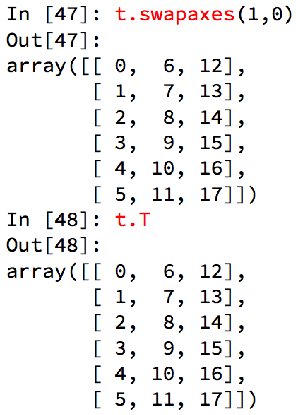
轴交换swapaxes

x :0 y:1 z:0
a.swapaxes(0,1)实际就是把x和y轴作为交换
a.swapaxes(1,1) 就是原来他们本身

>>> a.swapaxes(0,1) 
array([[ 0,  6, 12, 18],
       [ 1,  7, 13, 19],
       [ 2,  8, 14, 20],
       [ 3,  9, 15, 21],
       [ 4, 10, 16, 22],
       [ 5, 11, 17, 23]])
>>> a.swapaxes(0,1).shape
(6, 4)
>>> a.swapaxes(1,1)       
array([[ 0,  1,  2,  3,  4,  5],
       [ 6,  7,  8,  9, 10, 11],
       [12, 13, 14, 15, 16, 17],
       [18, 19, 20, 21, 22, 23]])

高维之间的转置

>>> c
array([[[ 0,  1,  2,  3,  4],
        [ 5,  6,  7,  8,  9]],

       [[10, 11, 12, 13, 14],
        [15, 16, 17, 18, 19]]])
>>> c.swapaxes(0,2)   
array([[[ 0, 10],
        [ 5, 15]],

       [[ 1, 11],
        [ 6, 16]],

       [[ 2, 12],
        [ 7, 17]],

       [[ 3, 13],
        [ 8, 18]],

       [[ 4, 14],
        [ 9, 19]]])
>>> c.swapaxes(0,2).shape
(5, 2, 2)
>>> c.swapaxes(1,2).shape 
(2, 5, 2)

轴对换之transpose

transpose进行的操作其实是将各个维度重置，默认对应的是（0,1,2）。使用transpose(1,0,2)后，其实就是将第一维和第二维互换。

>>> a
array([[ 0,  1,  2,  3,  4,  5], 
       [ 6,  7,  8,  9, 10, 11], 
       [12, 13, 14, 15, 16, 17], 
       [18, 19, 20, 21, 22, 23]])
>>> a.shape
(4, 6)
>>> a.transpose(1,0) 
array([[ 0,  6, 12, 18],
       [ 1,  7, 13, 19],
       [ 2,  8, 14, 20],
       [ 3,  9, 15, 21],
       [ 4, 10, 16, 22],
       [ 5, 11, 17, 23]])
>>> a.transpose(0,1) 
array([[ 0,  1,  2,  3,  4,  5],
       [ 6,  7,  8,  9, 10, 11],
       [12, 13, 14, 15, 16, 17],
       [18, 19, 20, 21, 22, 23]])

>>> d.transpose(0,1,2,3)   
array([[[[ 0,  1,  2],
         [ 3,  4,  5]],

        [[ 6,  7,  8],
         [ 9, 10, 11]]],


       [[[12, 13, 14],
         [15, 16, 17]],

        [[18, 19, 20],
         [21, 22, 23]]]])
>>> d.transpose(0,2,3,1)      
array([[[[ 0,  6],
         [ 1,  7],
         [ 2,  8]],

        [[ 3,  9],
         [ 4, 10],
         [ 5, 11]]],


       [[[12, 18],
         [13, 19],
         [14, 20]],

        [[15, 21],
         [16, 22],
         [17, 23]]]])

transpose和swapaxes的区别

相比之下transpose,更好应对了高维度的需求
T方法更简便高效的完成的特殊的需求

>>> a.swapaxes.__doc__
'a.swapaxes(axis1, axis2)\n\n    Return a view of the array with `axis1` and `axis2` interchanged.\n\n    Refer to `numpy.swapaxes` for full documentation.\n\n    See Also\n    --------\n    numpy.swapaxes : equivalent function'
>>> a.transpose.__doc__
'a.transpose(*axes)\n\n    Returns a view of the array with axes transposed.\n\n    For a 1-D array this has no effect, as a transposed vector is simply the\n    same vector. To convert a 1-D array into a 2D column vector, an additional\n    dimension must be added. `np.atleast2d(a).T` achieves this, as does\n    `a[:, np.newaxis]`.\n    For a 2-D array, this is a standard matrix transpose.\n    For an n-D array, if axes are given, their order indicates how the\n    axes are permuted (see Examples). If axes are not provided and\n    ``a.shape = (i[0], i[1], ... i[n-2], i[n-1])``, then\n    ``a.transpose().shape = (i[n-1], i[n-2], ... i[1], i[0])``.\n\n    Parameters\n    ----------\n    axes : None, tuple of ints, or `n` ints\n\n     * None or no argument: reverses the order of the axes.\n\n     * tuple of ints: `i` in the `j`-th place in the tuple means `a`\'s\n       `i`-th axis becomes `a.transpose()`\'s `j`-th axis.\n\n     * `n` ints: same 
as an n-tuple of the same ints (this form is\n       intended simply as a "convenience" alternative to the tuple form)\n\n    Returns\n  
  -------\n    out : ndarray\n        View of `a`, with axes suitably permuted.\n\n    See Also\n    --------\n    ndarray.T : Array property returning the array transposed.\n    ndarray.reshape : Give a new shape to an array without changing its data.\n\n    Examples\n    
--------\n    >>> a = np.array([[1, 2], [3, 4]])\n    >>> a\n    array([[1, 2],\n           [3, 4]])\n    >>> a.transpose()\n    array([[1, 3],\n           [2, 4]])\n    >>> a.transpose((1, 0))\n    array([[1, 3],\n           [2, 4]])\n    >>> a.transpose(1, 0)\n    array([[1, 3],\n           [2, 4]])'
>>>

八,视图和复制

a=b 完全不复制，a和b相互影响
a = b[:],视图的操作，一种切片，会创建新的对象a，但是a的数据完全由b保管，他们两个的数据变化是一致的，
a = b.copy(),复制，a和b互不影响

后续还有很多如,数组接口,排序,api,常量等等各种,后续在发