sofasofa——足球运动员身价估计

一、简介

1.背景介绍

每个足球运动员在转会市场都有各自的价码。本次数据练习的目的是根据球员的各项信息和能力值来预测该球员的市场价值。

2.数据

• 数据文件
  train.csv 训练集，文件大小 2.20mb
  test.csv 预测集, 文件大小 1.44kb
  sample_submit.csv 提交示例 文件大小 62kb
• 数据来源
  FIFA2018。为了公平起见，数据已经进行脱敏加工处理。
• 数据说明
  训练集中共有10441条样本，预测集中有7000条样本。每条样本代表一位球员，数据中每个球员有63项属性。数据中含有缺失值。
• 数据下载
  下载链接：http://sofasofa.io/competition.php?id=7传送门

3.变量说明

变量名	释义
id	行编号，没有实际意义
club	该球员所属的俱乐部。该信息已经被编码
league	该球员所在的联赛。已被编码
birth_date	生日。格式为月/日/年
height_cm	身高（厘米）
weight_kg	体重（公斤）
nationality	国籍；已被编码
potential	球员的潜力；数值变量
pac	球员速度；数值变量
sho	射门（能力值）；数值变量
pas	传球（能力值）；数值变量
dri	带球（能力值）；数值变量
def	防守（能力值）；数值变量
phy	身体对抗（能力值）；数值变量
international_reputation	国际知名度；数值变量
skill_moves	技巧动作；数值变量
weak_foot	非惯用脚的能力值；数值变量
work_rate_att	球员进攻的倾向。分类变量，Low, Medium, High
work_rate_def	球员防守的倾向。分类变量，Low, Medium, High
preferred_foot	惯用脚。1表示右脚、2表示左脚。
crossing	传中（能力值）。数值变量
finishing	完成射门（能力值）。数值变量
heading_accuracy	头球精度（能力值）。数值变量
short_passing	短传（能力值）。数值变量
volleys	凌空球（能力值）。数值变量
dribbling	盘带（能力值）。数值变量
curve	弧线（能力值）。数值变量
free_kick_accuracy	定位球精度（能力值）。数值变量
long_passing	长传（能力值）。数值变量
ball_control	控球（能力值）。数值变量
acceleration	加速度（能力值）。数值变量
sprint_speed	冲刺速度（能力值）。数值变量
agility	灵活性（能力值）。数值变量
reactions	反应（能力值）。数值变量
balance	身体协调（能力值）。数值变量
shot_power	射门力量（能力值）。数值变量
jumping	弹跳（能力值）。数值变量
stamina	体能（能力值）。数值变量
strength	力量（能力值）。数值变量
long_shots	远射（能力值）。数值变量
aggression	侵略性（能力值）。数值变量
interceptions	拦截（能力值）。数值变量
positioning	位置感（能力值）。数值变量
vision	视野（能力值）。数值变量
penalties	罚点球（能力值）。数值变量
marking	卡位（能力值）。数值变量
standing_tackle	断球（能力值）。数值变量
sliding_tackle	铲球（能力值）。数值变量
gk_diving	门将扑救（能力值）。数值变量
gk_handling	门将控球（能力值）。数值变量
gk_kicking	门将开球（能力值）。数值变量
gk_positioning	门将位置感（能力值）。数值变量
gk_reflexes	门将反应（能力值）。数值变量
rw	球员在右边锋位置的能力值。数值变量
rb	球员在右后卫位置的能力值。数值变量
st	球员在射手位置的能力值。数值变量
lw	球员在左边锋位置的能力值。数值变量
cf	球员在锋线位置的能力值。数值变量
cam	球员在前腰位置的能力值。数值变量
cm	球员在中场位置的能力值。数值变量
cdm	球员在后腰位置的能力值。数值变量
cb	球员在中后卫的能力值。数值变量
lb	球员在左后卫置的能力值。数值变量
gk	球员在守门员的能力值。数值变量
y	该球员的市场价值（单位为万欧元）。这是要被预测的数值

4.评价方法

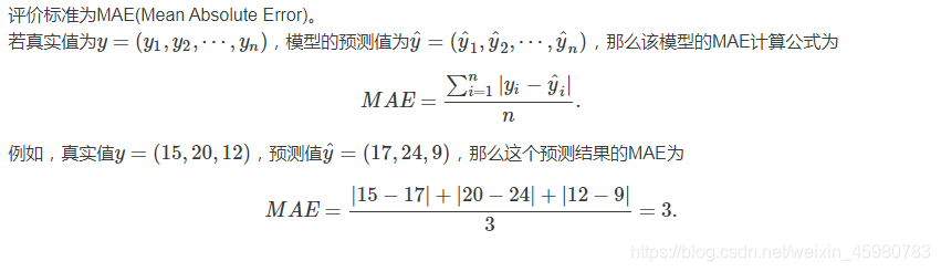
• MAE越小，说明模型预测得越准确。

二、标杆模型

官方给了两个标杆模型：http://sofasofa.io/benchmarks.php?id=7传送门

1.门将/非门将随机森林(Python)

import pandas as pd
import numpy as np
from datetime import date
from sklearn.ensemble import RandomForestRegressor


# 读取数据
train = pd.read_csv('train.csv')
test = pd.read_csv('test.csv')
submit = pd.read_csv('sample_submit.csv')


# 获得球员年龄
today = date(2018, 4, 15)

train['birth_date'] = pd.to_datetime(train['birth_date'])
train['age'] = (today - train['birth_date']).apply(lambda x: x.days) / 365.

test['birth_date'] = pd.to_datetime(test['birth_date'])
test['age'] = (today - test['birth_date']).apply(lambda x: x.days) / 365.


# 获得球员最擅长位置上的评分
positions = ['rw', 'rb', 'st', 'lw', 'cf', 'cam', 'cm', 'cdm', 'cb', 'lb', 'gk']

train['best_pos'] = train[positions].max(axis=1)
test['best_pos'] = test[positions].max(axis=1)


# 计算球员的身体质量指数(BMI)
train['BMI'] = 10000. * train['weight_kg'] / (train['height_cm'] ** 2)
test['BMI'] = 10000. * test['weight_kg'] / (test['height_cm'] ** 2)


# 判断一个球员是否是守门员
train['is_gk'] = train['gk'] > 0
test['is_gk'] = test['gk'] > 0


# 用多个变量准备训练随机森林
test['pred'] = 0
cols = ['height_cm', 'weight_kg', 'potential', 'BMI', 'pac',
        'phy', 'international_reputation', 'age', 'best_pos']


# 用非守门员数据训练随机森林
reg_ngk = RandomForestRegressor(random_state=100)
reg_ngk.fit(train[train['is_gk'] == False][cols], train[train['is_gk'] == False]['y'])

preds = reg_ngk.predict(test[test['is_gk'] == False][cols])
test.loc[test['is_gk'] == False, 'pred'] = preds


# 用守门员数据训练随机森林
reg_gk = RandomForestRegressor(random_state=100)
reg_gk.fit(train[train['is_gk'] == True][cols], train[train['is_gk'] == True]['y'])

preds = reg_gk.predict(test[test['is_gk'] == True][cols])
test.loc[test['is_gk'] == True, 'pred'] = preds


# 输出预测值
submit['y'] = np.array(test['pred'])
submit.to_csv('my_RF_prediction.csv', index=False)

门将/非门将随机森林——预测结果的MAE为：26.7350

2.四个变量的决策树模型(Python)

import pandas as pd
import numpy as np
from datetime import date
from sklearn.tree import DecisionTreeRegressor


# 读取数据
train = pd.read_csv('train.csv')
test = pd.read_csv('test.csv')
submit = pd.read_csv('sample_submit.csv')


# 获得球员年龄
today = date(2018, 4, 15)

train['birth_date'] = pd.to_datetime(train['birth_date'])
train['age'] = (today - train['birth_date']).apply(lambda x: x.days) / 365.

test['birth_date'] = pd.to_datetime(test['birth_date'])
test['age'] = (today - test['birth_date']).apply(lambda x: x.days) / 365.


# 获得球员最擅长位置上的评分
positions = ['rw', 'rb', 'st', 'lw', 'cf', 'cam', 'cm', 'cdm', 'cb', 'lb', 'gk']

train['best_pos'] = train[positions].max(axis=1)
test['best_pos'] = test[positions].max(axis=1)


# 用‘潜力’，‘国际知名度’，‘年龄’，‘最擅长位置评分’这四个变量来建立决策树模型
cols = ['potential', 'international_reputation', 'age', 'best_pos']

reg = DecisionTreeRegressor(random_state=100)
reg.fit(train[cols], train['y'])


# 输出预测值
submit['y'] = reg.predict(test[cols])
submit.to_csv('my_DT_prediction.csv', index=False)

四个变量的决策树模型——预测结果的MAE为：39.0321

3.总结

因为该比赛的评价方法是通过计算MAE进行比较。根据给出的两个不同的模型和其MAE值，可以知道门将/非门将随机森林模型的MAE是两个模型里最低的，所以我们试着先对该模型进行处理。

三、数据预处理

1.缺失值

代码：

print(train.info())

结果：

2.重复值

代码：

train.drop_duplicates(subset=None,keep='first',inplace=True)
print(train)

结果：

3.观察变量信息

代码：

print(train.describe())

结果：

4.相关系数查看

代码：

#导入numpy库	
#补充在在最开始导入库的版块里
import numpy as np

#格式：corr=文件名.corr
#0.2只是我的建议范围，波动范围在0.0~1.0
corr = train.corr()
corr[np.abs(corr) < 0.2] = np.nan		#绝对值低于0.2的就用nan替代
print(corr)

结果：

5.分类数据处理

1. 对于定量特征，其包含的有效信息为区间划分，例如本文中work_rate_att 和 work_rate_def 他们分别代表了球员进攻的倾向和球员防守的倾向。用Low，Medium，High表示。所以我们可能会将其转化为0 ，1，2 。
2. 代码：

 # 处理非数值型数据
label_mapping = {
        'Low':0,
        'Medium':1,
        'High':2
    }
traindata['work_rate_att'] = traindata['work_rate_att'].map(label_mapping)
traindata['work_rate_def'] = traindata['work_rate_def'].map(label_mapping)

6.缺失值

统计缺失值——代码：

train.isnull().sum(axis=0)	

处理缺失值——代码

train.fillna(method='backfill')			#用后面的值替换

可以用sklearn里的均值进行替换，但我用的时候报的错解决不了，决定用pandas解决

思前想后还是选择把缺失值进行删除：

train.dropna(axis=0,inplace=True)
train.isnull().sum(axis=0)

7.将出生日期转化为年龄

代码：

# 将出生年月日转化为年龄
traindata['birth_date'] = pd.to_datetime(traindata['birth_date'])
import datetime as dt

# 获取当前的年份
new_year = dt.datetime.today().year
traindata['birth_date'] = new_year - traindata.birth_date.dt.year

格式转换：

转换成年龄后：

8.身高体重转换为BMI指数

代码：

# 计算球员的身体质量指数（BMI）
train['BMI'] = 10000. * train['weight_kg'] / (train['height_cm'] ** 2)
test['BMI'] = 10000. * test['weight_kg'] / (test['height_cm'] ** 2)

9.将球员各个位置上的评分转化为球员最擅长位置的评分

代码：

# 获得球员最擅长位置上的评分
positions = ['rw','rb','st','lw','cf','cam','cm','cdm','cb','lb','gk']
 
train['best_pos'] = train[positions].max(axis =1)
test['best_pos'] = test[positions].max(axis = 1)

四、特征选择

1.归一化处理

代码：

if __name__ == '__main__':
    #### 读数据
    train_, test_ = getData()
    train,test = data_ana(train_,test_)

    #### 数据预处理
    minn = train['y'].min(axis=0)
    maxx = train['y'].max(axis=0)
    train['yy'] = train['y'].apply(lambda x: (x - minn)/(maxx - minn))
    train = train.drop('y',axis=1)

    # 字符串特征转换为数字特征
    work_rate_columns = ['work_rate_att', 'work_rate_def']
    for i in work_rate_columns:
        train[i] = pd.factorize(train[i])[0].astype(np.uint16)

    for i in work_rate_columns:
        test[i] = pd.factorize(test[i])[0].astype(np.uint16)

    # 生日转换
    today = date.today().year
    train['birth_date'] = pd.to_datetime(train['birth_date'])
    train['age'] = today - train.birth_date.dt.year
    test['birth_date'] = pd.to_datetime(test['birth_date'])
    test['age'] = today - test.birth_date.dt.year
    train = train.drop('birth_date', axis=1)
    test = test.drop('birth_date', axis=1)

    #### 特征工程
    # 归一化
    mm = MinMaxScaler()
    _data = mm.fit_transform(train)

2.过滤式

from sklearn.feature_selection import VarianceThreshold
import pandas as pd
 
def minmax_demo():
    """
    过滤低方差值
    :return:
    """
    #1 获取数据
    data=pd.read_csv(r"E:\my code\train.csv")
    data=data.iloc[:,:3]
    #print("data:\n",data)
    #2 实例化转换器  threshold方差值设定
    transfer=VarianceThreshold(threshold=10)
 
    #3 调用fit_transform
    data_new=transfer.fit_transform(data)
    print("data_new:\n",data_new,data_new.shape)
 
if __name__ == '__main__':
    minmax_demo()

结果：

不适合这次的数据，不选择用

3.删除低方差的特征

代码：

    # 特征选择：删除低方差的特征
    var = VarianceThreshold(threshold=1.0)  # 默认是删除 threshold=0 的特征，即删除重复数据
    try:
        _data = var.fit_transform(_data)
    except Exception as e:
        print('删除低方差的特征存在报错:', e)

    _data = pd.DataFrame(_data)
    _data.columns = train.columns.values
    train = _data

    # 缺失值填充
    train = train.fillna(0)
    print(train.isnull().any())

4.特征筛选

    #### 特征筛选
    cols = train.columns.values.tolist()
    cols.pop(cols.index('yy'))
    print("开始特征筛选")
    feature_ = xgboost_select_feature(train.drop(['yy'], axis=1), train['yy'], cols, 'yy')
    # feature_ = ['potential', 'best_pos', 'reactions', 'club', 'long_passing', 'BMI', 'vision', 'heading_accuracy', 'st', 'nationality', 'stamina', 'cf', 'aggression', 'free_kick_accuracy', 'pas', 'finishing', 'crossing', 'phy', 'marking']

特征工程结果 ：

五、模型的选择和调参

1.随机森林

根据官方给出的标杆模型，我初步选择的是随机森林的模型：

import pandas as pd
import numpy as np
import datetime as dt
from sklearn.ensemble import RandomForestRegressor

train = pd.read_csv(r"E:\my code\train.csv")
test = pd.read_csv(r"E:\my code\test.csv")
submit = pd.read_csv(r"E:\my code\sample_submit.csv")

# 获得球员年龄
today = dt.datetime.today().year

train['birth_date'] = pd.to_datetime(train['birth_date'])
train['age'] = today - train.birth_date.dt.year

test['birth_date'] = pd.to_datetime(test['birth_date'])
test['age'] = today - test.birth_date.dt.year

# 获取球员最擅长位置的评分
positions = ['rw','rb','st','lw','cf','cam','cm','cdm','cb','lb','gk']

train['best_pos'] = train[positions].max(axis=1)
test['best_pos'] = test[positions].max(axis=1)

# 计算球员的身体质量指数（BMI）
train['BMI'] = 10000. * train['weight_kg'] / (train['height_cm'] ** 2)
test['BMI'] = 10000. * test['weight_kg'] / (test['height_cm'] ** 2)

# 判断一个球员是否是守门员
train['is_gk'] = train['gk'] > 0
test['is_gk'] = test['gk'] > 0

# 用多个变量准备训练随机森林
test['pred'] = 0
cols =  ['height_cm', 'weight_kg', 'potential', 'BMI', 'pac',
        'phy', 'international_reputation', 'age', 'best_pos']

# 用非守门员的数据训练随机森林
# 使用网格搜索微调模型
from sklearn.model_selection import GridSearchCV
param_grid = [
    {'n_estimators':[3,10,30], 'max_features':[2,4,6,8]},
    {'bootstrap':[False], 'n_estimators':[3,10],'max_features':[2,3,4]}
]
forest_reg = RandomForestRegressor()
grid_search = GridSearchCV(forest_reg, param_grid ,cv=5,
                           scoring='neg_mean_squared_error')

grid_search.fit(train[train['is_gk'] == False][cols] , train[train['is_gk'] == False]['y'])

preds = grid_search.predict(test[test['is_gk'] == False][cols])
test.loc[test['is_gk'] == False , 'pred'] = preds

# 用守门员的数据训练随机森林
# 使用网格搜索微调模型
from sklearn.model_selection import GridSearchCV

param_grid1 = [
    {'n_estimators':[3,10,30], 'max_features':[2,4,6,8]},
    {'bootstrap':[False], 'n_estimators':[3,10],'max_features':[2,3,4]}
]

forest_reg1 = RandomForestRegressor()
grid_search1 = GridSearchCV(forest_reg, param_grid1 ,cv=5,
                           scoring='neg_mean_squared_error')

grid_search1.fit(train[train['is_gk'] == True][cols] , train[train['is_gk'] == True]['y'])

preds = grid_search1.predict(test[test['is_gk'] == True][cols])
test.loc[test['is_gk'] == True , 'pred'] = preds

# 输出预测值
submit['y'] = np.array(test['pred'])
submit.to_csv('my_RF_prediction1.csv',index = False)

# 打印参数的最佳组合
print(grid_search.best_params_)

结果：


提升的不太明显。

耍了个小聪明，之前做过的一次一次练习赛和这次一样，类型都是回归，而上一次练习用的就是xgboost模型，效果很好，所以这一次也用xgboost。


完整代码：

import pandas as pd
import numpy as np
from datetime import date
from sklearn.ensemble import RandomForestRegressor
from xgboost import XGBRegressor
from xgboost import plot_importance
import xgboost as xgb
from sklearn.model_selection import train_test_split
from pandas import Series, DataFrame
from sklearn.model_selection import train_test_split,cross_val_predict,cross_val_score, ShuffleSplit
from sklearn.model_selection import GridSearchCV,KFold
import matplotlib.pylab as plt
from matplotlib.pyplot import savefig
from matplotlib.pylab import rcParams
from sklearn.impute import SimpleImputer        # 均值填充
from xgboost import XGBRegressor, plot_importance
import time
from datetime import date
from sklearn.model_selection import GridSearchCV
import sklearn.metrics as metrics
from sklearn.feature_selection import VarianceThreshold
from sklearn.decomposition import PCA
from sklearn.preprocessing import MinMaxScaler


def getData():
    train = pd.read_csv(r"E:\my code\train.csv")
    test = pd.read_csv(r"E:\my code\test.csv")
    return train, test

def result_(test_res):
    submit = pd.read_csv(r"E:\my code\sample_submit.csv")
    submit['y'] = np.array(test_res)
    submit.to_csv('xiaoge5.csv', index=False)

def data_ana(train, test):

    # 获得球员最擅长位置上的评分
    positions = ['rw', 'rb', 'st', 'lw', 'cf', 'cam', 'cm', 'cdm', 'cb', 'lb', 'gk']

    train['best_pos'] = train[positions].max(axis=1)
    test['best_pos'] = test[positions].max(axis=1)


    # 计算球员的身体质量指数(BMI)
    train['BMI'] = 10000. * train['weight_kg'] / (train['height_cm'] ** 2)
    test['BMI'] = 10000. * test['weight_kg'] / (test['height_cm'] ** 2)

    # 判断一个球员是否是守门员
    train['is_gk'] = train['gk'].apply(lambda x: 1 if x > 0 else 0)
    test['is_gk'] = test['gk'].apply(lambda x: 1 if x > 0 else 0)

    return train,test


def modelfit(alg, data, labels_, cols, target, useTrainCV=True, cv_folds=7, early_stopping_rounds=50):
    if useTrainCV:
        xgb_param = alg.get_xgb_params()
        xgtrain = xgb.DMatrix(data, label=labels_)
        cvresult = xgb.cv(xgb_param, xgtrain, num_boost_round=alg.get_params()['n_estimators'], nfold=cv_folds,
            metrics='mae', early_stopping_rounds=early_stopping_rounds)
        alg.set_params(n_estimators=cvresult.shape[0])
        print('cv获得的最佳参数为:', cvresult.shape[0])
    #Fit the algorithm on the data
    seed = 20
    test_size = 0.3
    x_train,x_test,y_train,y_test = train_test_split(data, labels_, test_size=test_size,random_state=seed)    
    eval_set = [(x_test,y_test)]
    alg.fit(x_train, y_train, early_stopping_rounds=early_stopping_rounds, eval_metric='mae',eval_set=eval_set,verbose=True)        
    dtrain_predictions = alg.predict(x_test)

    y_true = list(y_test)
    y_pred = list(dtrain_predictions)

    #Print model report:
    print("\nModel Report")
    print("r2_score : %.4g" % metrics.r2_score(y_true, y_pred))
    mae_y = 0.00
    for i in range(len(y_true)):
        mae_y += np.abs(np.float(y_true[i])-y_pred[i])
    feat_imp = pd.Series(alg.get_booster().get_fscore()).sort_values(ascending=False)

    fig, ax = plt.subplots(1, 1, figsize=(8, 13))    
    plot_importance(alg, max_num_features=25, height=0.5, ax=ax)
    plt.show()
    plt.close()
    # 重要性筛选
    feat_sel = list(feat_imp.index)
    feat_val = list(feat_imp.values)
    featur = []
    for i in range(len(feat_sel)):
        featur.append([cols[int(feat_sel[i][1:])],feat_val[i]])
    print('所有特征的score:\n',featur)

    feat_sel2 = list(feat_imp[feat_imp.values > target].index)
    featur2 = []
    for i in range(len(feat_sel2)):
        featur2.append(cols[int(feat_sel2[i][1:])])    
    return featur2
    
def MAE_(xgb1,train_x,train_y):
    y_pre = list(xgb1.predict(train_x))
    train_y = train_y.values
    mae = metrics.median_absolute_error(train_y, y_pre)
    return mae

def xgboost_select_feature(data_, labels_,cols,target):# # 特征选择
    xgb1 = XGBRegressor(learning_rate =0.1,max_depth=5,min_child_weight=1,n_estimators=1000,
                    gamma=0,subsample=0.8,colsample_bytree=0.8,objective= 'reg:logistic',
                        nthread=4,scale_pos_weight=1,seed=27)       
    feature_ = list(modelfit(xgb1, data_.values, labels_.values, cols, 10)) # 特征选择
    return feature_


def xgboost_train(train_x, train_y):    
    train_x = train_x.values
    xgb1 = XGBRegressor(learning_rate=0.1, n_estimators=366, max_depth=24, min_child_weight=1, subsample=0.95,colsample_bytree=0.9,
                       gamma=0.1,objective= 'reg:logistic', nthread=4, seed=27)
    xgb1.fit(train_x,train_y)
    mae = MAE_(xgb1,train_x,train_y)
    print('在训练集上的mae为', mae)
    return xgb1

if __name__ == '__main__':
    #### 读数据
    train_, test_ = getData()
    train,test = data_ana(train_,test_)

    #### 数据预处理
    minn = train['y'].min(axis=0)
    maxx = train['y'].max(axis=0)
    train['yy'] = train['y'].apply(lambda x: (x - minn)/(maxx - minn))
    train = train.drop('y',axis=1)

    # 字符串特征转换为数字特征
    work_rate_columns = ['work_rate_att', 'work_rate_def']
    for i in work_rate_columns:
        train[i] = pd.factorize(train[i])[0].astype(np.uint16)

    for i in work_rate_columns:
        test[i] = pd.factorize(test[i])[0].astype(np.uint16)

    # 生日转换
    today = date.today().year
    train['birth_date'] = pd.to_datetime(train['birth_date'])
    train['age'] = today - train.birth_date.dt.year
    test['birth_date'] = pd.to_datetime(test['birth_date'])
    test['age'] = today - test.birth_date.dt.year
    train = train.drop('birth_date', axis=1)
    test = test.drop('birth_date', axis=1)

    #### 特征工程
    # 归一化
    mm = MinMaxScaler()
    _data = mm.fit_transform(train)

    # 特征选择：删除低方差的特征
    var = VarianceThreshold(threshold=1.0)  # 默认是删除 threshold=0 的特征，即删除重复数据
    try:
        _data = var.fit_transform(_data)
    except Exception as e:
        print('删除低方差的特征存在报错:', e)

    _data = pd.DataFrame(_data)
    _data.columns = train.columns.values
    train = _data

    # 缺失值填充
    train = train.fillna(0)
    print(train.isnull().any())

    #### 特征筛选
    cols = train.columns.values.tolist()
    cols.pop(cols.index('yy'))
    print("开始特征筛选")
    feature_ = xgboost_select_feature(train.drop(['yy'], axis=1), train['yy'], cols, 'yy')
    # feature_ = ['potential', 'best_pos', 'reactions', 'club', 'long_passing', 'BMI', 'vision', 'heading_accuracy', 'st', 'nationality', 'stamina', 'cf', 'aggression', 'free_kick_accuracy', 'pas', 'finishing', 'crossing', 'phy', 'marking']

    ##### train-------------------
    train = train.loc[:, feature_]
    xgb_ = XGBRegressor()
    xgb_ = xgboost_train(train.iloc[:,:train.shape[1]-1], train.iloc[:,train.shape[1]-1:])
    ##### predict-------------------
    feature_.pop()
    test = test[feature_]
    test = test.values      
    test_pre = xgb_.predict(test)
    test_pre_ = pd.DataFrame(test_pre).apply(lambda x: (maxx - minn)*x + minn)
    result_(test_pre_)

调参后结果：

在模型加入特征工程后：

特征工程没做好，没选好方法的反面教材本人

六、参考文章

1. https://www.cnblogs.com/wj-1314/p/10469240.html跳转
2. https://blog.csdn.net/weixin_41599977/article/details/89419373跳转
3. https://blog.csdn.net/xfei365/article/details/105128896跳转
4. https://www.jianshu.com/p/d6d243903a81跳转
5. https://blog.csdn.net/weixin_41261833/article/details/103589518跳转
6. https://blog.csdn.net/ACBattle/article/details/86218163跳转