


Explanation of radar signal processing algorithm implementation by Matlab
This blog documented the implementation of signal processing algorithms in my undergraduate graduation project. The content in this blog accounts for about 50% of the total project content of the graduation project
This blog lasted for two weeks, about 30h
Thanks to my teacher’s project, my peers’ inspiration, my friends’ encouragement, and my own persistence, I completed my graduation design
Chapter 1 Read in data
Chapter 2 Lowpass filter algorithm flowchart

Chapter 3 Bandpass filter algorithm flowchart

Chapter 4 Short-time fourier transform algorithms flowchart

Chapter 5 Wavelet transform algorithms flowchart
Chapter
- Explanation of radar signal processing algorithm implementation by Matlab
- 一、Read in data
- 二、Data preprocessing
- 三、Butterworth bandpass filter
- 3.1 Butterworth bandpass filter Matlab code
- 3.2 Matlab code for bandpass filter breathing
- 3.3 Matlab code for bandpass filter heartbeat
- 3.4 Bandpass filter test code
- 3.5 Test code of frequency domain plot by Fast Fourier Transform (FFT)
- 3.5.1 Matlab code for bandpass filter of Fast Fourier Transform (FFT)
- 3.5.2 Frequency domain plot illustrate
- 3.5.3 Frequency domain plot 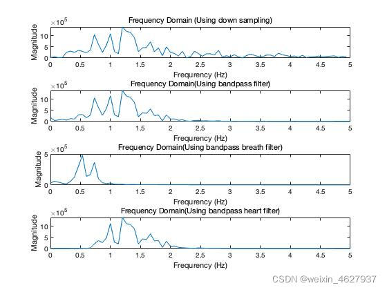
- 3.5.4 Solve the problem of cardiopulmonary signal separation
- 3.5.5 Summary
- 四. Short Time Fourier Transform(STFT)
- 五. Wavelet transform
- Summary
Introduction
In this project, we built a vital signs estimation system, using intelligent sensors and adding artificial intelligence algorithms to obtain human vital signs information. Use radar for data acquisition, proficiency in the use of matlab to achieve conventional signal processing, including: sampling, filtering, Fourier transform, short-term Fourier transform, wavelet transform, etc.
一、Read in data
Matlab code:
cd /Users/jiaoyexiang/Documents/MATLAB
filename1 = './test4radar.csv';
filename2 = csvread(filename1);
filename2 = filename2 - 32500*ones(15000,1);
raw_phase_signal = filename2;
二、Data preprocessing
2.1 Butterworth lowpass filter 1
2.1.1 Lowpass filter 1 Matlab code
function filter_phase_signal2 = siglowpassfilter(raw_phase_signal)

% A Butterworth lowpass filter 1 is designed as below

wp = 0.1/100; % Passband boundary frequency
ws = 0.3/100; % Stop band cutoff frequency
rp = 1; % Pass band fluctuations is 1dB
rs = 3; % The minimum stop band attenuation is 3 dB

[N, Wn] = buttord(wp,ws,rp,rs); % N is the filter order, Wn is the cut-off frequency
[b, a] = butter(N, Wn, 'low'); % design a lowpass filter and obtain the filter coefficients
filter_phase_signal2 = filter(b,a,raw_phase_signal); % filter() fliter function of matlab

end
2.2 Butterworth lowpass filter 2
2.2.1 Lowpass filter 2 Matlab code
function filter_phase_signal3 = siglowpassfilter2(raw_phase_signal)

% A Butterworth lowpass filter 2 is designed as below

wp = 0.01/100; % Passband boundary frequency
ws = 0.03/100; % Stop band cutoff frequency
rp = 1; % Pass band fluctuations is 1dB
rs = 3; % The minimum stop band attenuation is 3 dB

[N, Wn] = buttord(wp,ws,rp,rs); % The value of N is chosen with respect to the sampling frequency
[b, a] = butter(N, Wn, 'low'); % design a lowpass filter and obtain the filter coefficients
filter_phase_signal3 = filter(b,a,raw_phase_signal); % filter() fliter function of matlab

end
2.3 Test code and draw
2.3.1 Matlab test code
subplot(4,1,1)
plot(raw_phase_signal) % Original signal time domain waveform
title("raw phase signal")
filter_phase_signal = raw_phase_signal;

filter_phase_signal2 = siglowpassfilter(filter_phase_signal);  % Filter 1 filtering the original signal
subplot(4,1,2)
plot(filter_phase_signal2)
title("low noise signal")

signal3 = siglowpassfilter2(filter_phase_signal); % Filter 2 filtering the original signal
subplot(4,1,3)
plot(signal3)
title("breath signal")

signal4= filter_phase_signal2 - signal3; % Filter 1 minus filter 2
subplot(4,1,4)
plot(signal4)
title("heart pluse signal")
2.3.2 Time domain signal waveform obtained after filtering:

Figure explain
- The first line is the raw, unprocessed signal
- The second line is the signal after low-pass filter 1 processing
- The third line is the signal after low-pass filter2
- The forth line is the heartbeat signal obtained by the output signal 1 minus the output signal 2
2.4 Optimize test code and draw
2.4.1 Optimize Matlab test code
subplot(4,1,1)
plot(raw_phase_signal) % Original signal time domain waveform
title("raw phase signal")
filter_phase_signal = raw_phase_signal;

filter_phase_signal2 = siglowpassfilter(filter_phase_signal);  % Filter 1 filtering the original signal
subplot(4,1,2)
plot(filter_phase_signal2)
title("low noise signal")

signal3 = siglowpassfilter2(filter_phase_signal2); % Filter 2 filtering the filter_phase_signal2
subplot(4,1,3)
plot(signal3)
title("breath signal")

signal4= filter_phase_signal2 - signal3; % Filter 1 minus filter 2
subplot(4,1,4)
plot(signal4)
title("heart pluse signal")
2.4.2 Time domain signal waveform obtained after lowpass optimized filtering

2.5 The result of the algorithm optimization
We can see that the second filter is smoother and more stable in terms of amplitude fluctuations than the first one.
tupian1##
2.5.1 The reason of the change
The reason for this is that the filter is essentially a convolution of the filter and the original signal, and the squared amplitude function of the butterworth filter has a long transition band, so only one filter will have a residual effect on the signal in the later band.
As we all know: the Chebyshev filter decays faster than the Butterworth filter in the transition band, but the amplitude-frequency characteristics of the frequency response are not as flat as the latter.

2.5.2 Summary
This optimization retains the advantages of the butterworth lowpass filter and reduces the impact of the disadvantages of the butterworth lowpass filter
三、Butterworth bandpass filter
3.1 Butterworth bandpass filter Matlab code
function output = bandpassfilter(raw_phase_signal)

%{
A Butterworth band-pass filter is designed with
upper and lower boundary frequencies of 0.2Hz and 2Hz, respectively
%}

Fs = 1000;
LP = 0.2; %low cutoff frequency(Hz)
HP = 2; %high cutoff frequency(Hz)
NyquistF = 1/2*Fs; % Nyquist Sampling theorem
[B,A] = butter(3,[LP/NyquistF HP/NyquistF]); %Butterworth 3rd order filter
output = filtfilt(B,A,raw_phase_signal); %filtfilt() fliter function of matlab

end
3.1.1 Optimisation section
In the filtering matlab code, as can be seen from the figure, unlike the previous low-pass filter filter() function, I changed to the filtfilt() filter function. The advantage is that filtfilt() does the filtering and achieves zero phase shift filtering. This is also part of the algorithm
3.1.2 Explanation of reasons
Zero phase shift filtering is achieved because the filtfilt() function performs a filter-flip-refilter-flip process, which proceeds as follows:
y = filtfilt(b,a,x) Zero-phase digital filtering is achieved by processing the input data x in the forward and reverse directions. After filtering the data forward, filtfilt reverses the filtered sequence and passes it through the filter again.
The result has the following characteristics:
- Zero phase distortion
- The filter transfer function is equal to the squared magnitude of the original filter transfer function
- The filter order is twice that of the filter specified by b and a
3.2 Matlab code for bandpass filter breathing
low cutoff frequency is 0.2 Hz and high cutoff frequency is 0.7 Hz
%Bandpass filter breathing
function output_breath = bandpass_breath(raw_phase_signal)

Fs = 1000;
LP = 0.2; % low cutoff frequency (Hz)
HP = 0.7; % high cutoff frequency (Hz)
NyquistF = 1/2*Fs;
[B,A] = butter(3,[LP/NyquistF HP/NyquistF]); % Butterworth 3rd order filter
output_breath = filtfilt(B,A,raw_phase_signal);

end
3.3 Matlab code for bandpass filter heartbeat
low cutoff frequency is 0.8 Hz and high cutoff frequency is 2 Hz
%Band-pass filtered heartbeat
function output_heart = bandpass_heart(raw_phase_signal)
Fs = 1000;
LP = 0.8; %low cutoff frequency (Hz)
HP = 2; % high cutoff frequency (Hz)
NyquistF = 1/2*Fs;
[B,A] = butter(3,[LP/NyquistF HP/NyquistF]); % Butterworth 3rd order filter
output_heart = filtfilt(B,A,raw_phase_signal);
end
3.4 Bandpass filter test code
3.4.1 Matlab code for bandpass filter
output = bandpassfilter(raw_phase_signal);
subplot(4,1,2)
plot(output)
title("filter bandpass signal")

output_breath = bandpass_breath(raw_phase_signal);
subplot(4,1,3)
plot(output_breath)
title("filter bandpass signal breath")

output_heart = bandpass_heart(raw_phase_signal);
subplot(4,1,4)
plot(output_heart)
title("filter bandpass signal heart")
3.4.2 Time domain signal waveform obtained after bandpass filtering

3.5 Test code of frequency domain plot by Fast Fourier Transform (FFT)
3.5.1 Matlab code for bandpass filter of Fast Fourier Transform (FFT)
y1 = fft(output);
f1 = (0:length(y1)-1)*freq/length(y1); % Creates a vector f corresponding to the signal sample in the frequency space
y1 = fftshift(y1); % Shift the center
f1 = (-n/2:n/2-1)*(freq/n);

y2 = fft(output_breath);
f2 = (0:length(y2)-1)*freq/length(y2);
y2 = fftshift(y2);
f2 = (-n/2:n/2-1)*(freq/n);

y3 = fft(output_heart);
f3 = (0:length(y3)-1)*freq/length(y3);
y3 = fftshift(y3);
f3 = (-n/2:n/2-1)*(freq/n);

y0 = fft(data1);
f0 = (0:length(y0)-1)*freq/100/length(y0);
y0 = fftshift(y0);
f0 = (-n2/2:n2/2-1)*(freq/100/n2);

figure(5)
subplot(4,1,1)
plot(f0,100*abs(y0))
xlabel('Frequrency (Hz)')
ylabel('Magnitude')
title('Frequency Domain (Using down sampling)')
xlim([0,5])

subplot(4,1,2)
plot(f1,abs(y1))
xlabel('Frequrency (Hz)')
ylabel('Magnitude')
title('Frequency Domain(Using bandpass filter)')
xlim([0,5])

subplot(4,1,3)
plot(f2,abs(y2))
xlabel('Frequrency (Hz)')
ylabel('Magnitude')
title('Frequency Domain(Using bandpass breath filter)')
xlim([0,5])

subplot(4,1,4)
plot(f3,abs(y3))
xlabel('Frequrency (Hz)')
ylabel('Magnitude')
title('Frequency Domain(Using bandpass heart filter)')
xlim([0,5])
3.5.2 Frequency domain plot illustrate
- The first line in the figure represents the spectrum of the original signal after using the downsampling theorem
- The second line of the figure represents the spectrum of the signal using a band-pass filter, resulting in a composite signal of breathing and heartbeat
- The third line in the figure represents the spectrum of the breath signal after using a bandpass breathing filter
- The fourth line in the figure represents the spectrum of the heartbeat signal after using a band-pass heartbeat filter
3.5.3 Frequency domain plot 
3.5.4 Solve the problem of cardiopulmonary signal separation
When radar detects life signals, it obtains a composite signal of breathing and heartbeat. Therefore, when estimating the signal, the two signals should be separated. The amplitude of the heartbeat signal is very weak, and the breathing signal is much stronger than the heartbeat signal, resulting in the heartbeat signal being difficult to separate. At the same time, the heartbeat signal is also drowned out by strong clutter. Since the radar function is nonlinear, the harmonics of the breathing signal and the heartbeat signal are easily intermodulated, which will increase the difficulty of separating the cardiopulmonary signal
3.5.5 Summary
By contrast in the figure, we can clearly see that the frequency signal outside the cutoff frequency of the band-pass filter is effectively removed, and by using the two separated band-pass filters, the problem of cardiopulmonary signal separation is well solved. The spectral separation of the breathing and heartbeat signals is well realized. By finding the frequency peak, the frequency of the person’s breathing and heartbeat can be obtained
四. Short Time Fourier Transform(STFT)
This section builds on the band-pass filter processing in Chapter 3 to further refine the signal processing method
4.1 Principle of the Short-time Fourier transform(STFT)
The short-time Fourier transform is a method of time-frequency analysis of non-stationary signals, and the short-term time is realized by multiplying the window function with the product of the non-stationary signal to be analyzed. The small window is applied to the signal, and the signal is transformed within the small window, thus reflecting the local characteristics of the signal.
4.2 Reasons to adopt STFT to analyze cardiopulmonary signaling
In real life, the human heart-lung signal frequency will change with time, not periodic changes, frequency will change with time, is not a stationary signal, the use of fast Fourier transform will have great limitations, so the effect of time-frequency analysis will be better. The short-term Fourier transform is a non-stationary signal analysis algorithm, and the time-frequency analysis effect is generally better when the spectral component is relatively simple and uncomplicated. In general, it was a good fit for our project.
4.3 Matlab code of STFT
4.3.1 Window function selection principle:
Window selection principle is to be able to observe the true volatility of the sign signal at the same time, but also to take into account the frequency resolution, in the case of different window functions, the main peak side interference will be different.
%% STFT
fs = 1000;  % Sampling Frequency 1KHz
t = 15; % t = 0:1/fs:1-1/fs;
n = 15000;
for wlen = [32,64]
    % Using the for loop, set a comparison of different window lengths.
    % The longer the window, the worse the resolution, and the better the frequency resolution
    hop=wlen/4; % The minimum step size for each translation is 1. The smaller the image, the better the time
    output =wkeep1(output,N+1*wlen); % Truncated in the middle
    h=hamming(wlen); % Set the window length of the Haiming window
    subplot(1,2,wlen/32)
    spectrogram(output,h,wlen-hop,N,fs);   % B is the frequency peak of column T in F row, and P is the corresponding energy spectral density
    name=['wlen=', int2str(wlen)];
    title(name)
end

4.3.2 The explain of the figure
In the selection process, I used the for cycle comparison observation window of 16, 32, 64, 96 windows, after comparison, finally found that in the 15s observation time, using the window observation time of 6.4s, Fourier transform length of 64 points, the resolution was significantly improved, and there was no significant resolution enhancement for other higher frequency clutter, the determination of the length of the observation window of heart rate and the determination process of the length of the observation window of the respiratory rate were similar, and the window with a length of 64 was also finally selected.
4.3.3 STFT to obtain the spectrum of the signal
When used without output parameters, the spectrum is automatically plotted; with output parameters, the short-time Fourier transform of the input signal is returned
spectrogram(x, window, noverlap, nfft, fs)
4.3.4 Code description
s = spectrogram(x, window, noverlap, nfft, fs)
- X indicates the input signal.
- Window indicates the window function; if the value of window is an integer, then the length of each segment of x being segmented is equal to window and the default Hamming window is used; if window is a vector, then the length of each segment being segmented is equal to length(window) and the input vector is the window function to be added.
- Overlap indicates the number of overlap points between the two segments; the value of overlap must be less than the window length; if no overlap is specified, the default is half the window length, i.e. 50% of the overlap.
- Nfft means the number of points of fft, the number of points of fft can be different from the window length, when this parameter is not specified, Matlab will take max(256, 2^(ceil(log2(length(window))))), that is, when the window length is less than 256, the number of points of fft is 256; when the window length is longer than 256, the number of points of fft is taken to be greater than the smallest integer power of 2 of the window length.
- Fs indicates the sampling rate, used to normalise the display for use.
4.3.5 STFT Energy Spectrum
s = spectrogram(output, 64, 63, 256, fs);
t = 15;
f = linspace(0, 5);
nfft = 256;
[s, f, t, p] =  spectrogram(output, 64, 63, 256, fs);
figure(1);
xlabel('Time(s)')
ylabel('Frequrency (Hz)')
title('Short-time Fourier transform time-frequency (STFS)')
imagesc(t, f, 20*log10((abs(s))));xlabel('Time'); ylabel('Freqency');
colorbar;
xlim([0,5])
title('Draw with S')
h=colorbar;
h.Label.String = 'Power/Frequency(dB/Hz)';

4.3.6 STFT Output variable
S - Short-time Fourier transform of the input signal x. Each of its columns contains an estimate of the frequency component of short-term local time, with time increasing along the columns and frequency increasing along the rows. If x is a complex signal of length Nx, then S is a complex matrix of nfft rows and k columns, where k depends on window. If window is a scalar, then k = fix((Nx-noverlap)/(window-noverlap)). If window is a vector, then k = fix((Nx-noverlap)/(length(window)-noverlap))
F - Using the F frequency vector in the input variable, the function will calculate a spectrogram at the frequency specified by F using the Goertzel method.
For a real signal x, the number of rows of S is (nfft/2+1) if nfft is even, or (nfft+1)/2 if nfft is odd, with the same number of columns as above.
The specified frequencies are rounded to the nearest DFT container (bin) associated with the signal resolution. In other uses of the nfft syntax, the short-time Fourier transform method will be used. For the F-vector in the return value, which is the rounded frequency, its length is equal to the number of rows of S.
T-The point in time at which the spectrogram is calculated, whose length is equal to k as defined above, and whose value is the midpoint of each segment into which it is divided.
P - Energy spectral density PSD (Power Spectral
Density), for real signals, P is the unilateral period estimate of the PSD of each segment; for complex signals, P is the bilateral PSD when the F frequency vector is specified.
4.4 STFT Spectrogram Results
4.4.1 Matlab code of Frequency Domain
output = bandpassfilter(raw_phase_signal);
windowlength = 0.050;
Fs = 1000;

figure(10)
Windows=hamming(64); % Hamming window function size setting
yWindows=output.*Windows'; % Add a window function
subplot(211)
plot(yWindows)
yfftWindows=fft(yWindows);
f1 = (0:length(yfftWindows)-1)*Fs/length(yfftWindows);
subplot(212)
plot(f1, abs(yfftWindows)); % Plot the spectrum
xlim([0,2])

figure(11)
Windows=hamming(64); % Hamming window function size setting
yWindows_b=output_breath.*Windows'; % Add a window function
subplot(211)
plot(yWindows_b)
yfftWindows_b=fft(yWindows_b);
f1 = (0:length(yfftWindows_b)-1)*Fs/length(yfftWindows_b);
subplot(212)
plot(f1, abs(yfftWindows_b)); % Plot the spectrum
xlim([0,2])

figure(12)
Windows=hamming(64); % Hamming window function size setting
yWindows_h=output_heart.*Windows';  % Add a window function
subplot(211)
plot(yWindows_h)
yfftWindows_h=fft(yWindows_h);
f1 = (0:length(yfftWindows_h)-1)*Fs/length(yfftWindows_h);
subplot(212)
plot(f1, abs(yfftWindows_h)); % Plot the spectrum
xlim([0,2])


4.5 Shortcomings of STFT
Although the STFT can improve the shortcomings of the Fourier transform to a certain extent and realise the time-frequency analysis of the signal, its time resolution is fixed and therefore cannot effectively reflect the sudden change of the signal, and its application is limited.
Wavelet analysis extends the STFT to achieve a new time-frequency analysis method, whose time window can shrink as the frequency of the signal increases and increase as the frequency decreases, effectively solving the short-time Fourier transform shortcomings of the signal, and is therefore widely used
五. Wavelet transform
This section builds on the band-pass filter processing in Chapter 3 and STFT transform in Chapter 4 to further refine the signal processing method
5.1 Wavelet concept
5.1.1 Wavelet definition
Waves in small areas, special length limited, mean 0
5.1.2 Wavelet feature
- Tightly branched or approximately tightly branched in the time domain
- Alternating positive and negative “volatility” with no DC component
5.1.3 Wavelet transform steps
- Take a wavelet and compare it with the top end of the signal
- Calculate the correlation factor C. The larger the C, the higher the correlation between the wavelet and the data.
- Move the wavelet and repeat steps 1 and 2, traversing the entire data
- Scale the wavelet, repeat steps 1 to 3, and repeat the above steps for all wavelet scales
5.2 Reasons to adopt Wavelet to analyze cardiopulmonary signaling
- The size and shape of the window function of the short-time Fourier transform is constant.
- Wavelet analysis extends the signal STFT and implements a new time-frequency analysis method, whose time window can shrink as the frequency of the signal increases and increase as the frequency decreases, effectively solving the shortcomings of STFT
5.3 Wavelet Signal Denoiser
5.3.1 Basic wavelet denoising methods
Generally speaking, the noise reduction process of a one-dimensional signal can be divided into 3 steps
- Wavelet decomposition of the signal. Select a wavelet and determine a level a of wavelet decomposition, then calculate A layers of wavelet decomposition for the signal.
- Threshold quantization of the high frequency coefficients of the wavelet decomposition. For each of the high frequency coefficients (three directions) from layer 1 to layer N, a threshold value is chosen for threshold quantization. This is the most critical step, mainly in the selection of the threshold and the quantization process. matlab provides a lot of adaptive methods for the selection of the threshold of each layer, which are not introduced here. The two different methods achieve the effect that the hard thresholding method can well preserve the local features such as signal edges, while the soft thresholding process is relatively smooth, but can cause distortions such as edge blurring.
figure(3)
c = cwt(output, 1:10, 'db2', 'plot');

- Wavelet reconstruction of the signal. Wavelet reconstruction of the signal is performed based on the low-frequency coefficients in layer N of the wavelet decomposition and the high-frequency coefficients in layers 1 to N after quantization.
5.3.2 Basic problem of wavelet threshold denoising
The basic problem of wavelet threshold denoising includes three aspects: the selection of wavelet bases, the selection of threshold values, and the selection of threshold functions.
- Wavelet base selection: usually we hope that the selected wavelets satisfy the following conditions: orthogonality, high vanishing moments, tight branching, symmetry or antisymmetry. But in fact the wavelet with the above properties is impossible to exist, because the wavelet is symmetric or antisymmetric only Haar wavelet, and high vanishing moment and tight support is a pair of contradictions, so in the application of the general selection of wavelets with tight support and according to the characteristics of the signal to select a more appropriate wavelet.
- Threshold selection: An important factor that directly affects the denoising effect is the selection of the threshold, different threshold selection will have different denoising effect. At present, there are mainly generic threshold values (VisuShrink), SureShrink threshold values, Minimax threshold values, BayesShrink threshold values, etc.
- Selection of the threshold function: The threshold function is the rule for correcting wavelet coefficients, and different inverse functions reflect different strategies for dealing with wavelet coefficients. The most commonly used threshold function has two kinds: one is a hard threshold function, the other is a soft threshold function. There is also a Garrote function which is in between the soft and hard threshold functions.
In addition, the signal-to-noise ratio (SNR) and the root mean square error (RMSE) of the estimated signal to the original signal are commonly used to evaluate the effectiveness of denoising.
Here, I choose symmetry as Wavelet selection, bayes as Threshold selection and a median function which is in between the soft and hard threshold function. The result of Wavelet Signal Denoiser is shown as below:
 Fig.1.1 Wavelet denoising of respiratory signals Fig.1.1 Wavelet denoising of respiratory signals
|
 Fig.1.2 Wavelet decomposition coefficients Fig.1.2 Wavelet decomposition coefficients
|
 Fig.2.1 Wavelet denoising of heartbeat signals Fig.2.1 Wavelet denoising of heartbeat signals
|
 Fig.2.2 Wavelet decomposition coefficients Fig.2.2 Wavelet decomposition coefficients
|
5.4 Matlab code for wavelet transform
fs = 1000;
t=0:1/fs:1;
wavename='cmor3-3';
Fc=centfrq(wavename); % The center frequency of the wavelet
totalscal=256;
c=2*Fc*totalscal;
scals=c./(1:totalscal);
f=scal2frq(scals,wavename,1/fs); % Converts scale to frequency
coefs=cwt(s,scals,wavename); % Find the continuous wavelet coefficient
figure
imagesc(t,f,abs(coefs));
set(gca,'YDir','normal')
colorbar;
xlabel('Time t/s');
ylabel('frequency f/Hz');
title('Wavelet time-frequency diagram');
5.4.1 Matlab code description
The three functions cwt(), centfrq(), scal2frq() in the wavelet toolbox that need to be used. The specific parameters and uses are described as follows.
(1) COEFS = cwt(S,SCALES,‘wname’)
This function implements the continuous wavelet transform, where S is the input signal, SCALES is the scale, and wname is the wavelet name.
(2) FREQ = centfrq(‘wname’)
The function seeks the centre frequency of the mother wavelet named by wname.
(3) F = scal2frq(A,‘wname’,DELTA)
The function can convert the scale to the actual frequency, where A is the scale, wname for the wavelet name, DELTA for the sampling period

5.4.2 Summary of Wavelet
In the figure, we see that the time-frequency aggregation reflected on the time-frequency plot of the wavelet transform is good
Summary
In the process of trying out new algorithms for signal processing, I learned more about how to use Matlab and learned to understand multiple functions, and I became proficient in a variety of signal processing methods. Although the new algorithms did not improve the correct rate by a large margin, I gained a lot by trying to apply it.
During the six months I studied in Suzhou, I not only learned a lot of professional knowledge and enriched my knowledge system, but I also made a lot of like-minded partners. It was the right decision to come to Suzhou and I will always be grateful. I would like to thank my teachers and seniors for their guidance and answering questions throughout the year, and I will continue to do my best to contribute to myself, my family, my school and society by being eager for knowledge and persistent for truth.


 3126
3126

 被折叠的 条评论
为什么被折叠?
被折叠的 条评论
为什么被折叠?
 到【灌水乐园】发言


