pyspark使用LinearRegression

Gadaite

于 2022-01-10 07:25:25 发布

阅读量1.1k

点赞数

文章标签： spark 大数据数据挖掘

本文链接：https://blog.csdn.net/weixin_46408961/article/details/122402972

版权

01.导入模块，创建对象

from pyspark.sql import SparkSession
from pyspark.ml.regression import LinearRegression
spark = SparkSession.builder.config("spark.driver.host","192.168.1.4")\
    .config("spark.ui.showConsoleProgress","false")\
    .appName("CruiseLinear").master("local[*]").getOrCreate()

02.加载数据查看结构：

data = spark.read.csv("/mnt/e/win_ubuntu/Code/DataSet/MLdataset/cruise_ship_info.csv",header=True,inferSchema=True)
data.printSchema()

输出结果：

root
 |-- Ship_name: string (nullable = true)
 |-- Cruise_line: string (nullable = true)
 |-- Age: integer (nullable = true)
 |-- Tonnage: double (nullable = true)
 |-- passengers: double (nullable = true)
 |-- length: double (nullable = true)
 |-- cabins: double (nullable = true)
 |-- passenger_density: double (nullable = true)
 |-- crew: double (nullable = true)

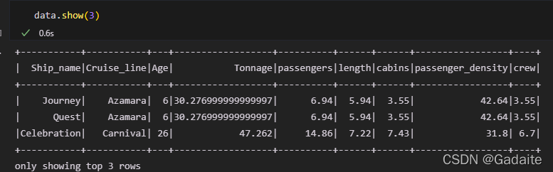
03.查看DF表的数据内容：

data.show(3)

输出结果：

04.按照Cruise_line进行分组计数，并进行从大到小排序：

from pyspark.sql.functions import desc
data.groupBy('Cruise_line').count().orderBy('count').sort(desc("count")).show()

输出结果：

+-----------------+-----+
|      Cruise_line|count|
+-----------------+-----+
|  Royal_Caribbean|   23|
|         Carnival|   22|
|         Princess|   17|
| Holland_American|   14|
|        Norwegian|   13|
|            Costa|   11|
|        Celebrity|   10|
|              MSC|    8|
|              P&O|    6|
|             Star|    6|
|Regent_Seven_Seas|    5|
|        Silversea|    4|
|           Cunard|    3|
|         Seabourn|    3|
|         Windstar|    3|
|          Oceania|    3|
|          Crystal|    2|
|           Disney|    2|
|          Azamara|    2|
|           Orient|    1|
+-----------------+-----+

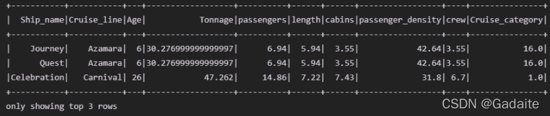
05.按照Cruise_line这一列类别进行特征（或标签）进行编码，使其数值化

from pyspark.ml.feature import StringIndexer
stringIndexer = StringIndexer(inputCol="Cruise_line",outputCol="Cruise_category")
model_one = stringIndexer.fit(data)
data = model_one.transform(data)
data.show(3)

输出结果：

06.对数据进行向量化：

选取：'Age', 'Tonnage', 'passengers', 'length', 'cabins', 'passenger_density', 'Cruise_category'

from pyspark.ml.feature import VectorAssembler
vectorAssembler = VectorAssembler(inputCols=['Age', 'Tonnage', 'passengers', 'length', 'cabins', 'passenger_density', 'Cruise_category']\
    ,outputCol="features")
data = vectorAssembler.transform(data)
data.show(3)

输出结果：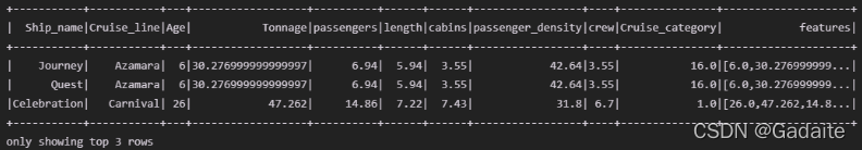

07.获取需要的数据即为：

data = data.select(["features","crew"])
data.show(3)

输出结果：

+--------------------+----+
|            features|crew|
+--------------------+----+
|[6.0,30.276999999...|3.55|
|[6.0,30.276999999...|3.55|
|[26.0,47.262,14.8...| 6.7|
+--------------------+----+

08.具体查看前3行的数据：

data.head(3)

输出结果：

[Row(features=DenseVector([6.0, 30.277, 6.94, 5.94, 3.55, 42.64, 16.0]), crew=3.55),
 Row(features=DenseVector([6.0, 30.277, 6.94, 5.94, 3.55, 42.64, 16.0]), crew=3.55),
 Row(features=DenseVector([26.0, 47.262, 14.86, 7.22, 7.43, 31.8, 1.0]), crew=6.7)]

09.拆分训练数据和测试数据数据：

原始数据的行数：

data.count()

输出结果：158

训练数据，测试数据拆分和行数查询：

datatrain,datatest = data.randomSplit([0.7,0.3])
print(datatrain.count(),datatest.count())

输出结果：109 49

10.查看训练数据的描述信息：

datatrain.describe().show()

输出结果：

+-------+------------------+
|summary|              crew|
+-------+------------------+
|  count|               109|
|   mean| 7.917431192660562|
| stddev|3.5179485298462865|
|    min|              0.59|
|    max|              21.0|
+-------+------------------+

11.查看预测数据描述信息：

datatest.describe().show()

输出结果：

+-------+------------------+
|summary|              crew|
+-------+------------------+
|  count|                49|
|   mean| 7.519999999999998|
| stddev|3.4914789130109316|
|    min|              0.59|
|    max|              13.6|
+-------+------------------+

12.使用训练数据构建线性回归模型，预测结果与原结果比对：

linearRegression = LinearRegression(labelCol="crew")
model_two = linearRegression.fit(datatrain)
train_res = model_two.transform(datatrain)
train_res.show(3)

输出结果：

+--------------------+----+------------------+
|            features|crew|        prediction|
+--------------------+----+------------------+
|[4.0,220.0,54.0,1...|21.0|20.910397653785616|
|[5.0,115.0,35.74,...|12.2|11.963885749291746|
|[5.0,122.0,28.5,1...| 6.7| 6.395983956954153|
+--------------------+----+------------------+
only showing top 3 rows

13.使用测试数据，对模型进行评估，生成测试结果：

res_test = model_two.evaluate(datatest)

14.查看测试结果的各种描述结果：

今天带来的内容是Error系列的指标及loss损失函数，该系列有：

均方误差（Mean Square Error，MSE）
平均绝对误差（Mean Absolute Error，MAE）
均方根误差（Root Mean Square Error，RMSE）
均方对数误差（Mean Squared Log Error）
平均相对误差（Mean Relative Error，MAE）

14.1：rootMeanSquaredError，别名RMSE，均方根误差(Root Mean Square Error)

res_test.rootMeanSquaredError

输出结果：0.8703930750875685

14.2：r2,比率

分子是均方误差，分母是方差

R2_score = 1，达到最大值。即分子为 0 ，意味着样本中预测值和真实值完全相等，没有任何误差

R2_score = 0，此时分子等于分母，样本的每项预测值都等于均值

R2_score < 0 ，分子大于分母，训练模型产生的误差比使用均值产生的还要大，也就是训练模型反而不如直接去均值效果好。通常是模型本身不是线性关系的，而我们误使用了线性模型，导致误差很大

res_test.r2

输出结果：0.9365594630744019

14.3：meanSquaredError，别名MSE，均方误差(Mean Square Error)

res_test.meanSquaredError

输出结果：0.7575841051603937

14.4：meanAbsoluteError，别名MAE，平均绝对误差(Mean Absolute Error)

res_test.meanAbsoluteError

输出结果：0.5771184769144841

15.加载一下原始数据：

oridata = spark.read.csv("/mnt/e/win_ubuntu/Code/DataSet/MLdataset/cruise_ship_info.csv",header=True,inferSchema=True)

16.引入sparksql函数中的corr相关系数模块，查询某两列的person相关系数

from pyspark.sql.functions import corr
oridata.select(corr('crew', 'passengers')).show()

输出结果：

+----------------------+
|corr(crew, passengers)|
+----------------------+
|    0.9152341306065384|
+----------------------+

oridata.select(corr('crew', 'cabins')).show()

输出结果：

+------------------+
|corr(crew, cabins)|
+------------------+
|0.9508226063578497|
+------------------+

Gadaite

关注

0
点赞
踩
10

收藏

觉得还不错? 一键收藏
0
评论
pyspark使用LinearRegression

01.导入模块，创建对象from pyspark.sql import SparkSessionfrom pyspark.ml.regression import LinearRegressionspark = SparkSession.builder.config("spark.driver.host","192.168.1.4")\ .config("spark.ui.showConsoleProgress","false")\ .appName("CruiseLinear")..
复制链接

扫一扫