


Developed by Ruofan Ding, Xudong Zou, Yangmei Qin, Gao Wang, Lei Li
xQTLbiolinks: a comprehensive and scalable tool for integrative analysis of molecular QTLs
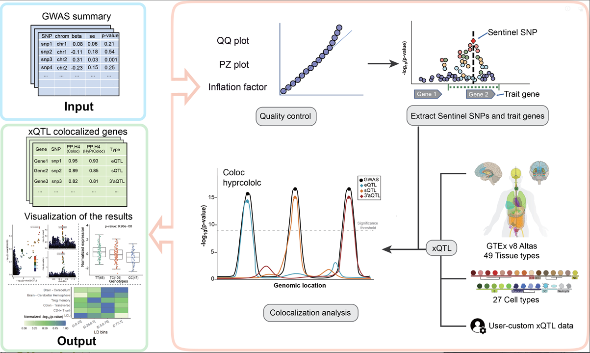
xQTLbiolinks is a end-to-end bioinformatic tool for efficient mining and analyzing public and user-customized xQTLs data for the discovery of disease susceptibility genes. xQTLbiolinks consists of tailored functions that can be grouped into four modules: Data retrieval, Pre-processing, Analysis and Visualization.
Instructions, documentation, and tutorials can be found at here.
Quick Start
xQTLbiolinkscan be installed and used on any operator systems supporting R. The latest version (v1.6.3) is also available at GitHub repository and it can be installed throughdevtools::install_github("dingruofan/xQTLbiolinks”). For more details, please refer to the instructions at Installation section below.- Find the Query and download for xQTLs, gene, variant, tissue, sample and expressions.
- Find the Quick Start for a quick application of colocalization analysis with xQTLbiolinks. Go through a whole Case study of detection of casual vairants and genes in prostate cancer using
xQTLbiolinks. - The details and instructions of all functions implemented in xQTLbiolinks can be found here. Find more instructions with examples for visualizations here.
Citation
If you find the xQTLbiolinks package or any of the source code in this repository useful for your work, please cite:
Ruofan Ding, Xudong Zou, Yangmei Qin, Lihai Gong, Hui Chen, Xuelian Ma, Shouhong Guang, Chen Yu, Gao Wang, Lei Li, xQTLbiolinks: a comprehensive and scalable tool for integrative analysis of molecular QTLs, Briefings in Bioinformatics, Volume 25, Issue 1, January 2024, bbad440,
Institute of Systems and Physical Biology, Shenzhen Bay Laboratory, Shenzhen 518055, China
Dependencies
The xQTLbiolinks package has the following dependencies:
R packages: BiocGenerics, cowplot (>= 1.1.1), curl (>= 4.3.2), data.table (>= 1.14.2), DBI, SummarizedExperiment, GenomeInfoDb, GenomicFeatures, GenomicRanges, ggplot2 (>= 3.3.6), ggrepel, IRanges, jsonlite (>= 1.7.2), viridis, RMySQL, stringr (>= 1.4.0), utils (>= 4.0.3),VariantAnnotation, TxDb.Hsapiens.UCSC.hg38.knownGene, PupillometryR, coloc, hyprcoloc, knitr, rtracklayer, usethis, ggridges, CMplot, R.utils, ggforestplot.
Installation
To install this R package, you will need to have required package SummarizedExperiment installed from Bioconductor with following command:
if (!require("BiocManager", quietly = TRUE)){install.packages("BiocManager")}
BiocManager::install("SummarizedExperiment") # For windows or linux
BiocManager::install("SummarizedExperiment",type="source") # For MAC
Once you have installed the required package, you can then install xQTLbiolinks from CRAN or github(recommended) using following command:
# Install from github to get the latest version.
if(!require("devtools")){install.packages("devtools")}
devtools::install_github("dingruofan/xQTLbiolinks")
2. A quick application of coloclization analysis
2023-05-01
Source: vignettes/Quick_start.Rmd
xQTLbiolinks has provided a pipeline for disease target gene discovery through colocalization analysis with xQTLs to detect susceptible genes and causal variants.
Before we start
To perform colocalization analysis using xQTLbiolinks, users need to provide their own GWAS summary statistics data, specify the tissue of interest and import following packages:
library(data.table)
library(xQTLbiolinks)
library(stringr)
library(coloc)
Step 1. data pre-processing
Download and load an example file of summary statistics dataset (GRCh38). We perform colocalization analysis in Brain - Cerebellum.
gwasDF <- fread("http://bioinfo.szbl.ac.cn/xQTL_biolinks/xqtl_data/gwasDFsub.txt")
tissueSiteDetail="Brain - Cerebellum"
In this example, a data.table object of 16538 (rows) x 5 (cols) is loaded. Five columns are required (arbitrary column names is supported, but columns must be as the following order):
Col 1. “variants” (character), , using an rsID (e.g. “rs11966562”);
Col 2. “chromosome” (character), one of the chromosome from chr1-chr22;
Col 3. “position” (integer), genome position of snp;
Col 4. “P-value” (numeric);
Col 5. “MAF” (numeric). Allel frequency;
Col 6. “beta” (numeric). effect size.
Col 7. “se” (numeric). standard error.
head(gwasDF)#> rsid chrom position pValue AF beta se
#> 1: rs13120565 4 10702513 5.66e-10 0.6429 0.01825 0.00294
#> 2: rs4697781 4 10703243 8.94e-10 0.6446 0.01803 0.00294
#> 3: rs4697779 4 10701187 5.74e-09 0.3231 -0.01747 0.00300
#> 4: rs4697780 4 10701381 5.95e-09 0.3231 -0.01746 0.00300
#> 5: rs4547789 4 10702891 1.46e-08 0.3197 -0.01703 0.00300
#> 6: rs11726285 4 10700944 1.47e-08 0.3214 -0.01702 0.00301Step 2. Identify sentinel snps.
Sentinel SNPs can be detected using xQTLanalyze_getSentinelSnp with the arguments p-value < 5e-8 and SNP-to-SNP distance > 10e6 bp. We recommend converting the genome version of the GWAS file to GRCh38 if that is GRCh37 (run with parameter: genomeVersion="grch37"; grch37To38=TRUE, and package rtracklayeris required).
sentinelSnpDF <- xQTLanalyze_getSentinelSnp(gwasDF, pValueThreshold = 5e-08)After filtering, a sentinel SNP with P-value<5e-8 is detected in this example:
sentinelSnpDF#> rsid chr position pValue maf beta se
#> 1: rs13120565 chr4 10702513 5.66e-10 0.6429 0.01825 0.00294Step 3. Identify trait genes for each sentinel SNPs.
Trait genes are genes that located in the range of 1Mb (default, can be changed with parameter detectRange) of sentinel SNPs. Every gene within 1Mb of sentinel SNPs is searched by fuction xQTLanalyze_getTraits. Besides, In order to reduce the number of trait genes and thus reduce the running time, we take the overlap of eGenes and trait genes as the final output of the function xQTLanalyze_getTraits.
traitsAll <- xQTLanalyze_getTraits(sentinelSnpDF, detectRange=1e6, tissueSiteDetail=tissueSiteDetail)Totally, 3 associations between 3 traits genes and 1 SNPs are detected
traitsAll#> rsid chr position pValue maf beta se gencodeId
#> 1: rs13120565 chr4 10702513 5.66e-10 0.6429 0.01825 0.00294 ENSG00000002587
#> 2: rs13120565 chr4 10702513 5.66e-10 0.6429 0.01825 0.00294 ENSG00000109684
#> 3: rs13120565 chr4 10702513 5.66e-10 0.6429 0.01825 0.00294 ENSG00000261490Step 4. Conduct colocalization analysis.
For a single trait gene, like ENSG00000109684 in above table, colocalization analysis (using coloc method) can be performed with:
output <- xQTLanalyze_coloc(gwasDF, "ENSG00000109684", tissueSiteDetail=tissueSiteDetail) # using gene symboloutput is a list, including two parts: coloc_Out_summary and gwasEqtlInfo.
output$coloc_Out_summary#> nsnps PP.H0.abf PP.H1.abf PP.H2.abf PP.H3.abf PP.H4.abf
#> 1: 7107 7.097893e-11 1.32221e-07 3.890211e-06 0.00625302 0.993743
#> traitGene candidate_snp SNP.PP.H4
#> 1: ENSG00000109684 rs13120565 0.5328849For multiple trait genes, a for loop or lapply function can be used to get all genes’ outputs (using both coloc and hyprcoloc methods).
outputs <- rbindlist(lapply( unique(traitsAll$gencodeId), function(x){ # using gencode ID.
xQTLanalyze_coloc(gwasDF, x, tissueSiteDetail=tissueSiteDetail, method = "Both")$colocOut }))outputs is a data.table that combined all results of coloc_Out_summary of all genes.
outputs#> traitGene nsnps PP.H0.abf PP.H1.abf PP.H2.abf PP.H3.abf
#> 1: ENSG00000002587 6452 1.730175e-05 3.218430e-02 6.603361e-05 0.12198838
#> 2: ENSG00000109684 7107 7.097893e-11 1.322210e-07 3.890211e-06 0.00625302
#> 3: ENSG00000261490 6601 5.287051e-05 9.848309e-02 4.801374e-04 0.89435622
#> PP.H4.abf candidate_snp SNP.PP.H4 hypr_posterior hypr_regional_prob
#> 1: 0.84574398 rs13120565 0.4140146 0.5685 0.9694
#> 2: 0.99374296 rs13120565 0.5328849 0.9793 0.9999
#> 3: 0.00662768 rs13120565 0.4219650 0.0000 0.0101
#> hypr_candidate_snp hypr_posterior_explainedBySnp
#> 1: rs13120565 0.2726
#> 2: rs13120565 0.4747
#> 3: rs13120565 0.4118Step 5. Visualization of the results.
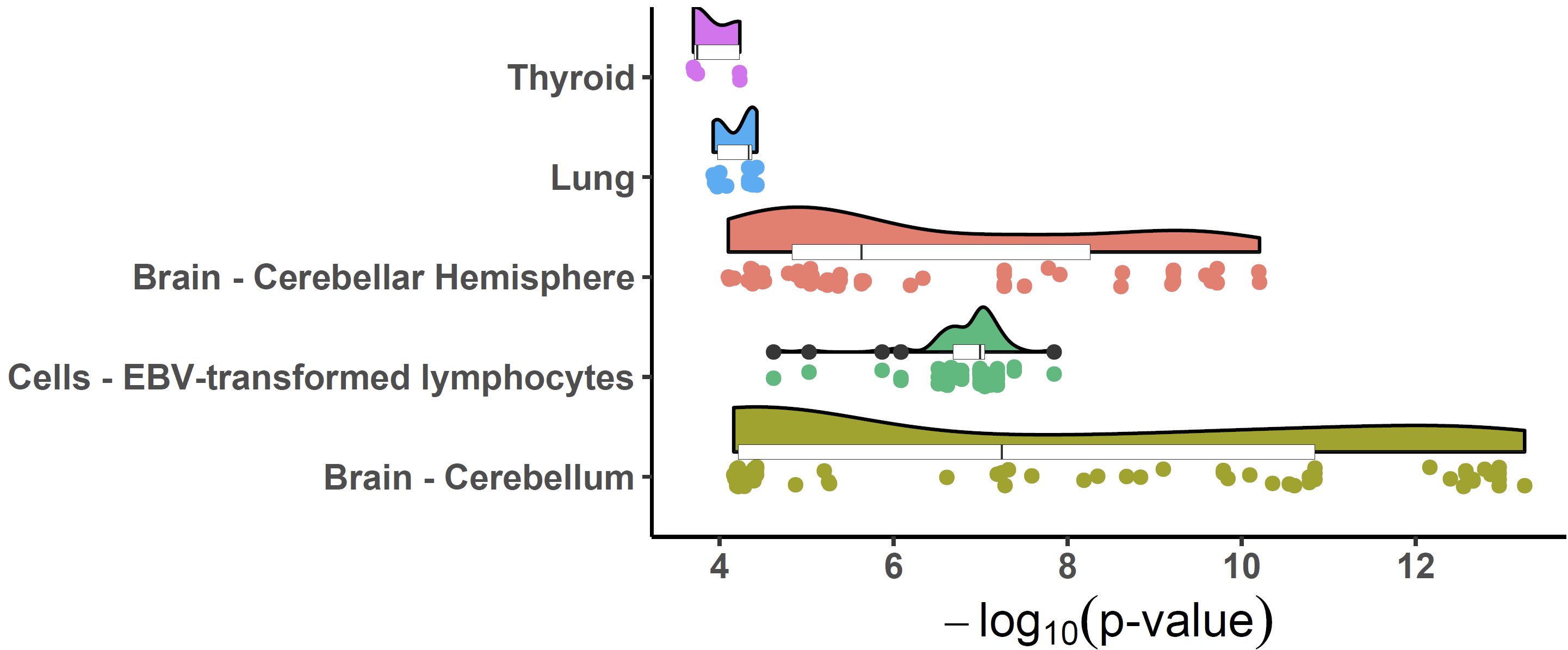
For the potential casual gene ENSG00000109684 (PP4=0.9937 & hypr_posterior=0.9999), we can get its significant associations across tissues:
xQTLvisual_eqtl("ENSG00000109684")
For the purpose of visualization of p-value distribution and comparison of the signals of GWAS and eQTL: We merge the variants of GWAS and eQTL by rsid first.
eqtlAsso <- xQTLdownload_eqtlAllAsso(gene="ENSG00000109684",
tissueLabel = tissueSiteDetail, data_source = "liLab")
gwasEqtldata <- merge(gwasDF, eqtlAsso, by="rsid", suffixes = c(".gwas",".eqtl"))Function xQTLvisual_locusCompare displays the candidate SNP rs13120565 (SNP.PP.H4=0.5328849 & hypr_posterior_explainedBySnp=0.4747) in the top right corner:
xQTLvisual_locusCompare(gwasEqtldata[,.(rsid, pValue.eqtl)],
gwasEqtldata[,.(rsid, pValue.gwas)], legend_position = "bottomright")Note: The information on SNP linkage disequilibrium is automatically downloaded online. Due to network issues, the download may fail at times. If this happens, please try running it again.

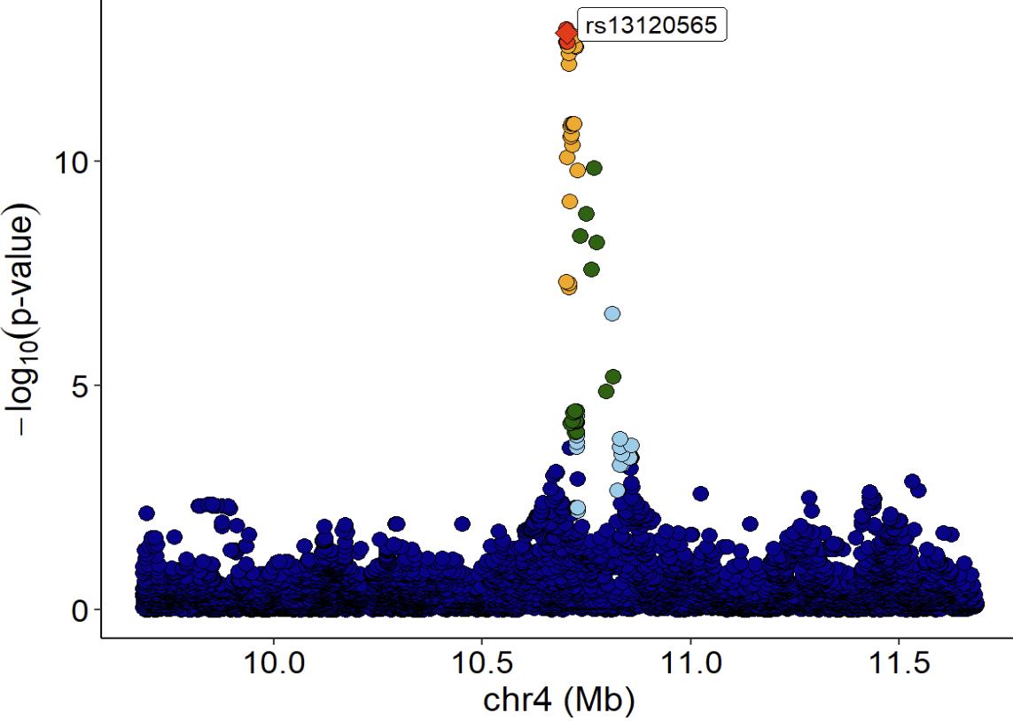
Locuszoom plot of GWAS signals:
xQTLvisual_locusZoom(gwasEqtldata[,.(rsid, chrom, position, pValue.gwas)], legend=FALSE)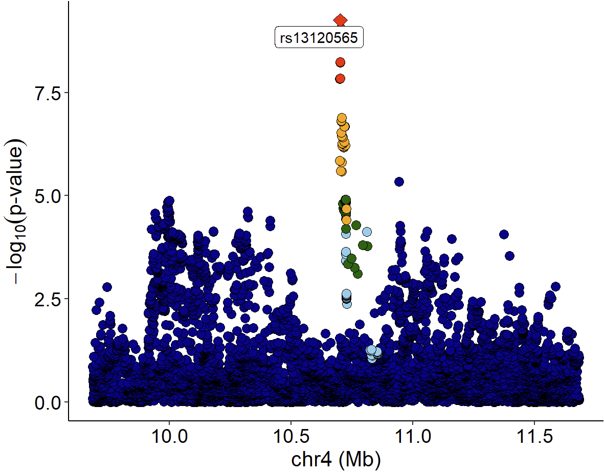
LocusZoom plot of eQTL signals:
xQTLvisual_locusZoom(gwasEqtldata[,.(rsid, chrom, position, pValue.eqtl)],
highlightSnp = "rs13120565", legend=FALSE)
Violin plot of normalized expression of eQTL (rs13120565-ENSG00000187323.11):
xQTLvisual_eqtlExp("rs13120565", "ENSG00000109684", tissueSiteDetail = tissueSiteDetail)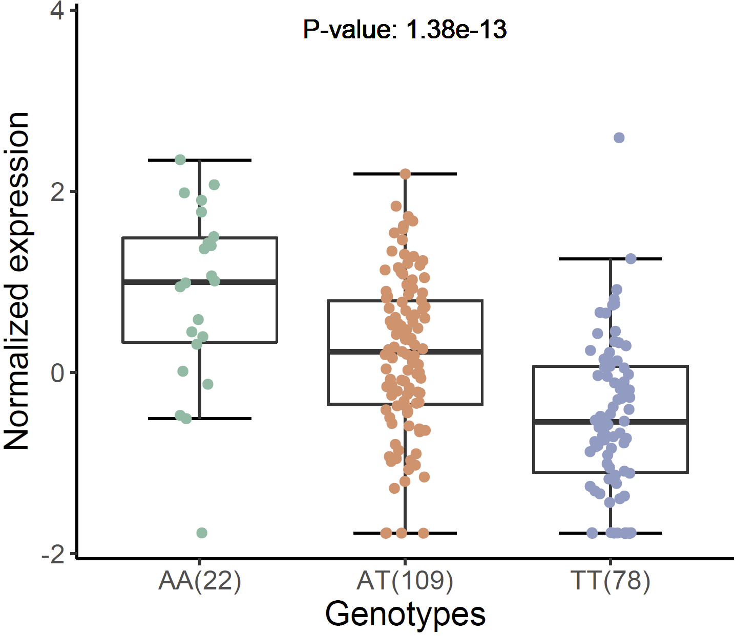
We can also combine locuscompare and locuszoom plot using xQTLvisual_locusCombine:
xQTLvisual_locusCombine(gwasEqtldata[,c("rsid","chrom", "position", "pValue.gwas", "pValue.eqtl")],
highlightSnp="rs13120565")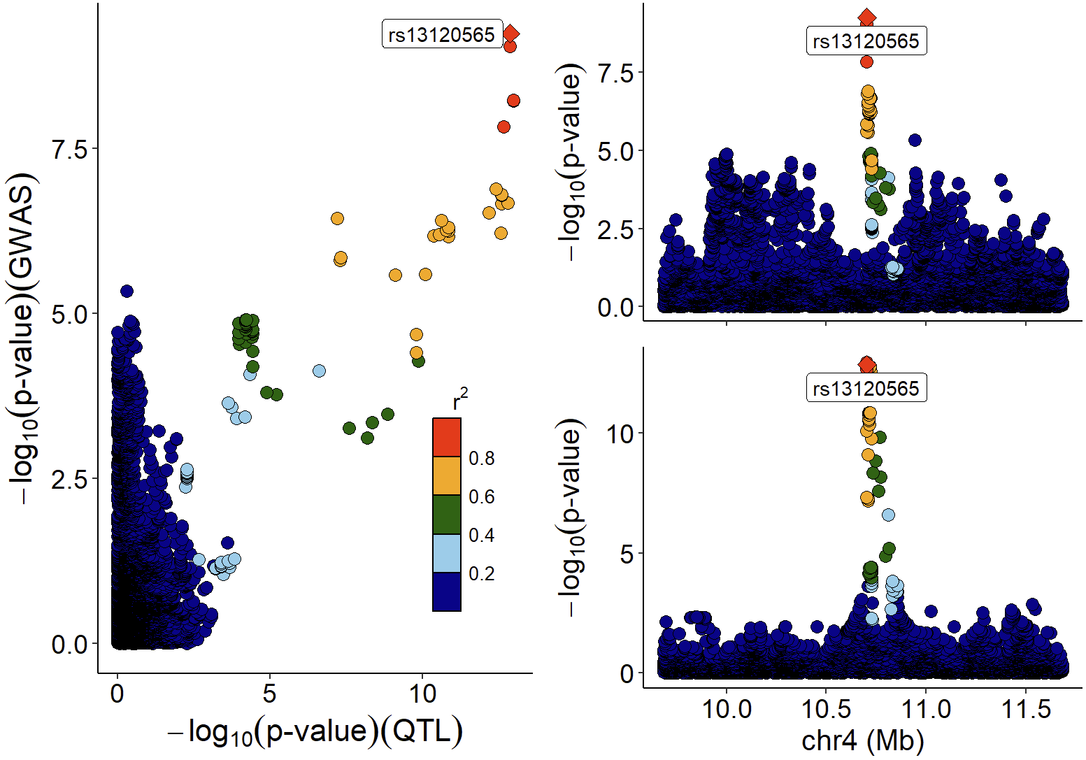
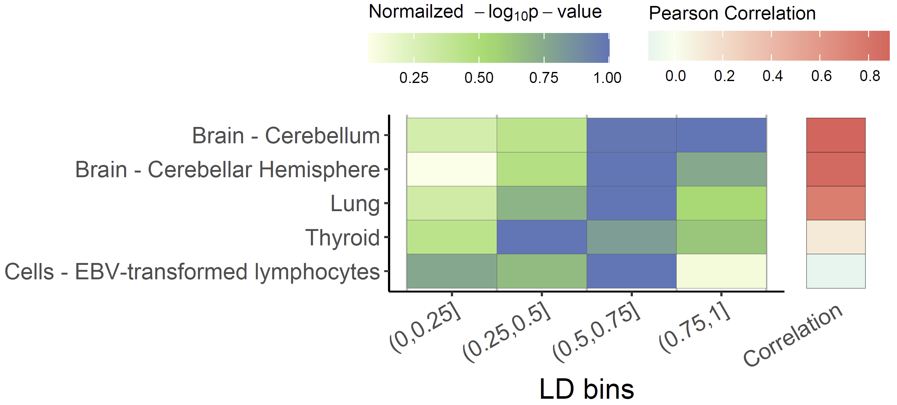
Colocalized loci should show a general pattern where SNPs in high LD will show strong associations with expression levels of the colocalized gene, and the eQTL associations will weaken for SNPs in lower LD. This pattern of the eQTL varies among different tissues / cell-types, the strength of which indicates the power of the regulatory effect of the variant. We can visualize the correlation between p-values of eQTLs and LD across numerous tissues/cell types to easily distinguish this patten using xQTLvisual_coloc:
multi_tissue_coloc <- xQTLvisual_coloc(gene="ENSG00000109684", variantName="rs13120565",
tissueLabels = c("Brain - Cerebellar Hemisphere",
"Brain - Cerebellum", "Thyroid", "Lung",
"Cells - EBV-transformed lymphocytes"))
For applying xQTLbiolinks to a whole case study, please find this Document.
2. A quick application of coloclization analysis
2. 归落分析的快速应用
Developed by Ruofan Ding, Xudong Zou, Yangmei Qin, Gao Wang, Lei Li.
开发者:Ruofan Ding, Xudong Zou, Yangmei Qin, Gao Wang, Lei Li.
2023-05-01
Source: vignettes/Quick_start.Rmd资料来源:vignettes/Quick_start。Rmd
xQTLbiolinks has provided a pipeline for disease target gene discovery through colocalization analysis with xQTLs to detect susceptible genes and causal variants.
xQTLbiolinks 通过与 xQTL 的共定位分析来检测易感基因和致病变异,为疾病靶基因发现提供了一条管道。

Before we start 开始之前
To perform colocalization analysis using xQTLbiolinks, users need to provide their own GWAS summary statistics data, specify the tissue of interest and import following packages:
要使用 xQTLbiolinks 进行共定位分析,用户需要提供自己的 GWAS 摘要统计数据,指定感兴趣的组织并导入以下软件包:
Step 1. data pre-processing
步骤 1.数据预处理
Download and load an example file of summary statistics dataset (GRCh38). We perform colocalization analysis in Brain - Cerebellum.
下载并加载汇总统计数据集 (GRCh38) 的示例文件。我们在 Brain - Cerebellum 中进行共定位分析。
In this example, a data.table object of 16538 (rows) x 5 (cols) is loaded. Five columns are required (arbitrary column names is supported, but columns must be as the following order):
在此示例中,加载了 16538 (rows) x 5 (cols) 的 data.table 对象。需要五列(支持任意列名,但列必须按以下顺序排列):
Col 1. “variants” (character), , using an rsID (e.g. “rs11966562”);列 1.“variants” (字符), , 使用 rsID (例如 “rs11966562”);
Col 2. “chromosome” (character), one of the chromosome from chr1-chr22;列 2.“chromosome” (character),来自 chr1-chr22 的染色体之一;
Col 3. “position” (integer), genome position of snp;列 3.“position” (整数),SNP 的基因组位置;
Col 4. “P-value” (numeric);列 4.“P 值”(数字);
Col 5. “MAF” (numeric). Allel frequency;列 5.“MAF” (数字)。等位基因频率;
Col 6. “beta” (numeric). effect size.列 6.“beta” (数字)。effect size 的 intent 值。
Col 7. “se” (numeric). standard error.列 7.“se” (数字)。标准误差。
#>          rsid chrom position   pValue     AF     beta      se
#> 1: rs13120565     4 10702513 5.66e-10 0.6429  0.01825 0.00294
#> 2:  rs4697781     4 10703243 8.94e-10 0.6446  0.01803 0.00294
#> 3:  rs4697779     4 10701187 5.74e-09 0.3231 -0.01747 0.00300
#> 4:  rs4697780     4 10701381 5.95e-09 0.3231 -0.01746 0.00300
#> 5:  rs4547789     4 10702891 1.46e-08 0.3197 -0.01703 0.00300
#> 6: rs11726285     4 10700944 1.47e-08 0.3214 -0.01702 0.00301
Step 2. Identify sentinel snps.
步骤 2。识别 sentinel snp。
Sentinel SNPs can be detected using xQTLanalyze_getSentinelSnp with the arguments p-value < 5e-8 and SNP-to-SNP distance > 10e6 bp. We recommend converting the genome version of the GWAS file to GRCh38 if that is GRCh37 (run with parameter: genomeVersion="grch37"; grch37To38=TRUE, and package rtracklayeris required).
可以使用带有参数 p 值 < 5e-8 和 SNP 到 SNP 距离 > 10e6 bp 的 xQTLanalyze_getSentinelSnp 来检测 Sentinel SNP。如果 GRCh37 是 GRCh37,我们建议将 GWAS 文件的基因组版本转换为 GRCh38(使用参数运行:genomeVersion=“grch37”;grch37To38=TRUE,并且需要打包 rtracklayer)。
After filtering, a sentinel SNP with P-value<5e-8 is detected in this example:
过滤后,在此示例中检测到 P 值为 <5e-8 的哨兵 SNP:
#>          rsid  chr position   pValue    maf    beta      se
#> 1: rs13120565 chr4 10702513 5.66e-10 0.6429 0.01825 0.00294
Step 3. Identify trait genes for each sentinel SNPs.
步骤 3。确定每个哨兵 SNP 的性状基因。
Trait genes are genes that located in the range of 1Mb (default, can be changed with parameter detectRange) of sentinel SNPs. Every gene within 1Mb of sentinel SNPs is searched by fuction xQTLanalyze_getTraits. Besides, In order to reduce the number of trait genes and thus reduce the running time, we take the overlap of eGenes and trait genes as the final output of the function xQTLanalyze_getTraits.
性状基因是位于哨兵 SNP 的 1Mb (默认,可以使用参数 detectRange 更改) 范围内的基因。前哨 SNP 的 1Mb 内的每个基因都通过功能xQTLanalyze_getTraits进行搜索。此外,为了减少性状基因的数量,从而减少运行时间,我们将 eGenes 和性状基因的重叠作为功能xQTLanalyze_getTraits的最终输出。
Totally, 3 associations between 3 traits genes and 1 SNPs are detected
总共检测到 3 个性状基因和 1 个 SNP 之间的 3 个关联
#>          rsid  chr position   pValue    maf    beta      se       gencodeId
#> 1: rs13120565 chr4 10702513 5.66e-10 0.6429 0.01825 0.00294 ENSG00000002587
#> 2: rs13120565 chr4 10702513 5.66e-10 0.6429 0.01825 0.00294 ENSG00000109684
#> 3: rs13120565 chr4 10702513 5.66e-10 0.6429 0.01825 0.00294 ENSG00000261490
Step 4. Conduct colocalization analysis.
步骤 4。进行共定位分析。
For a single trait gene, like ENSG00000109684 in above table, colocalization analysis (using coloc method) can be performed with:
对于单个性状基因,如上表中ENSG00000109684,可以通过以下方式进行共定位分析(使用 coloc 方法):
output is a list, including two parts: coloc_Out_summary and gwasEqtlInfo.
output 是一个列表,包括 coloc_Out_summary 和 gwasEqtlInfo 两部分。
#>    nsnps    PP.H0.abf   PP.H1.abf    PP.H2.abf  PP.H3.abf PP.H4.abf
#> 1:  7107 7.097893e-11 1.32221e-07 3.890211e-06 0.00625302  0.993743
#>          traitGene candidate_snp SNP.PP.H4
#> 1: ENSG00000109684    rs13120565 0.5328849
For multiple trait genes, a for loop or lapply function can be used to get all genes’ outputs (using both coloc and hyprcoloc methods).
对于多个性状基因,可以使用 for 循环或 lapply 函数来获取所有基因的输出(使用 coloc 和 hyprcoloc 方法)。
outputs is a data.table that combined all results of coloc_Out_summary of all genes.
outputs 是一个 data.table,它结合了所有基因的 coloc_Out_summary 的所有结果。
#>          traitGene nsnps    PP.H0.abf    PP.H1.abf    PP.H2.abf  PP.H3.abf
#> 1: ENSG00000002587  6452 1.730175e-05 3.218430e-02 6.603361e-05 0.12198838
#> 2: ENSG00000109684  7107 7.097893e-11 1.322210e-07 3.890211e-06 0.00625302
#> 3: ENSG00000261490  6601 5.287051e-05 9.848309e-02 4.801374e-04 0.89435622
#>     PP.H4.abf candidate_snp SNP.PP.H4 hypr_posterior hypr_regional_prob
#> 1: 0.84574398    rs13120565 0.4140146         0.5685             0.9694
#> 2: 0.99374296    rs13120565 0.5328849         0.9793             0.9999
#> 3: 0.00662768    rs13120565 0.4219650         0.0000             0.0101
#>    hypr_candidate_snp hypr_posterior_explainedBySnp
#> 1:         rs13120565                        0.2726
#> 2:         rs13120565                        0.4747
#> 3:         rs13120565                        0.4118
Step 5. Visualization of the results.
步骤 5。结果的可视化。
For the potential casual gene ENSG00000109684 (PP4=0.9937 & hypr_posterior=0.9999), we can get its significant associations across tissues:
对于潜在的偶然基因ENSG00000109684(PP4=0.9937 & hypr_posterior=0.9999),我们可以得到它在组织中的显著关联:
For the purpose of visualization of p-value distribution and comparison of the signals of GWAS and eQTL: We merge the variants of GWAS and eQTL by rsid first.
为了可视化 p 值分布和比较 GWAS 和 eQTL 的信号:我们首先通过 rsid 合并 GWAS 和 eQTL 的变体。
Function xQTLvisual_locusCompare displays the candidate SNP rs13120565 (SNP.PP.H4=0.5328849 & hypr_posterior_explainedBySnp=0.4747) in the top right corner:
函数xQTLvisual_locusCompare在右上角显示候选SNP rs13120565 (SNP.PP.H4=0.5328849 & hypr_posterior_explainedBySnp=0.4747):
Note: The information on SNP linkage disequilibrium is automatically downloaded online. Due to network issues, the download may fail at times. If this happens, please try running it again.
注意: 有关 SNP 连锁不平衡的信息可自动在线下载。由于网络问题,下载有时可能会失败。如果发生这种情况,请尝试再次运行它。

Locuszoom plot of GWAS signals:
GWAS 信号的 Locuszoom 图:

LocusZoom plot of eQTL signals:
eQTL 信号的 LocusZoom 图:
Violin plot of normalized expression of eQTL (rs13120565-ENSG00000187323.11):
eQTL 归一化表达的小提琴图 (rs13120565-ENSG00000187323.11):

We can also combine locuscompare and locuszoom plot using xQTLvisual_locusCombine:
我们还可以使用 xQTLvisual_locusCombine 组合 locuscompare 和 locuszoom 图:

Colocalized loci should show a general pattern where SNPs in high LD will show strong associations with expression levels of the colocalized gene, and the eQTL associations will weaken for SNPs in lower LD. This pattern of the eQTL varies among different tissues / cell-types, the strength of which indicates the power of the regulatory effect of the variant. We can visualize the correlation between p-values of eQTLs and LD across numerous tissues/cell types to easily distinguish this patten using xQTLvisual_coloc:
共定位位点应显示一种一般模式,其中高 LD 中的 SNP 将与共定位基因的表达水平表现出很强的相关性,而低 LD 中 SNP 的 eQTL 关联将减弱。eQTL 的这种模式在不同的组织/细胞类型中有所不同,其强度表明变体的调节作用的强度。我们可以可视化多种组织/细胞类型中 eQTL 和 LD 的 p 值之间的相关性,以便使用 xQTLvisual_coloc 轻松区分这种模式:
For applying xQTLbiolinks to a whole case study, please find this Document.
有关将 xQTLbiolinks 应用于整个案例研究,请查找此文档。
Developed by Ruofan Ding, Xudong Zou, Yangmei Qin, Gao Wang, Lei Li.
开发者:Ruofan Ding, Xudong Zou, Yangmei Qin, Gao Wang, Lei Li.


 被折叠的 条评论
为什么被折叠?
被折叠的 条评论
为什么被折叠?
 到【灌水乐园】发言


