


 本文以Kaggle房价预测任务为例,详细阐述了数据预处理和特征工程的步骤。包括了解数据集基本信息、处理缺失值、分析目标变量与特征间关系、数据变换(如Box-Cox变换)以解决异方差性,以及特征选择和编码策略。通过这些方法,可以提升模型预测性能。
文章目录
引言
以Kaggle房价回归预测为例,来叙述回归问题中数据预处理与特征工程的一般流程,这是参考公开notebook的,觉得人家写的很条理,不像自己的都拼西凑。刚买了《python数据分析与挖掘实战》,希望系统的学习一下!
一、数据预处理
1.数据集的基本信息
加载数据集
# 加载数据集
train = pd.read_csv('../input/house-prices-advanced-regression-techniques/train.csv',header=0,index_col=0)
test = pd.read_csv('../input/house-prices-advanced-regression-techniques/test.csv',header=0,index_col=0)
# 以 f开头表示在字符串内支持大括号内的python 表达式,与常见的以r开头是同一类用法,只不过以r开头是去掉反斜杠机制
print (f"Train has {train.shape[0]} rows and {train.shape[1]} columns")
print (f"Test has {test.shape[0]} rows and {test.shape[1]} columns")
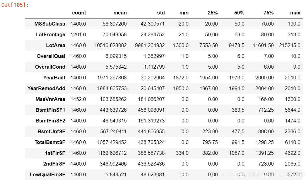
关于数值变量的统计信息
# 这里的转置是因为变量比较多,转置后方便观察
train.describe().T
对所有特征变量的属性,内存等信息的统计
train.info()

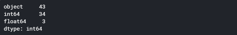
统计不同类型对象的个数
train.dtypes.value_counts()
2.缺失值统计及可视化
使用missingno进行缺失值可视化,训练集与测试集分别进行
mg.matrix(train)

统计每个变量的缺失比例
# 定义一个统计每个变量缺失比例的函数
def missing_percentage(df):
    total = df.isnull().sum().sort_values(ascending = False)[df.isnull().sum().sort_values(ascending = False) != 0]
    percentage = round(df.isnull().sum().sort_values(ascending=False)*100 / len(df),2)[df.isnull().sum().sort_values(ascending=False)*100 / len(df) != 0]
    return pd.concat([total,percentage],axis = 1,keys=['Total','Percentage'])

missing_percentage(train)

3.变量分析
3.1目标变量的分析
分析目标标量,建立直方图与连续概率估计图,数据和正态分布分位数的拟合图,箱型图
def plot_1(df,feature):
    # 一种图的格式
    style.use('fivethirtyeight')
    fig,axes = plt.subplots(3,1,constrained_layout=True,figsize=(10,24))
    # 画直方图与连续概率密度估计图
    # norm_hist=True:如果为True,则直方图的高度显示密度而不是计数
    sns.distplot(df.loc[:,feature],norm_hist=True,ax=axes[0])

    # 通过比较数据和正态分布的分位数是否相等来判断数据是不是符合正态分布
    stats.probplot(df.loc[:,feature],plot=axes[1])

    # 箱型图
    sns.boxplot(df.loc[:,feature],orient='h',ax=axes[2])

plot_1(train,'SalePrice')

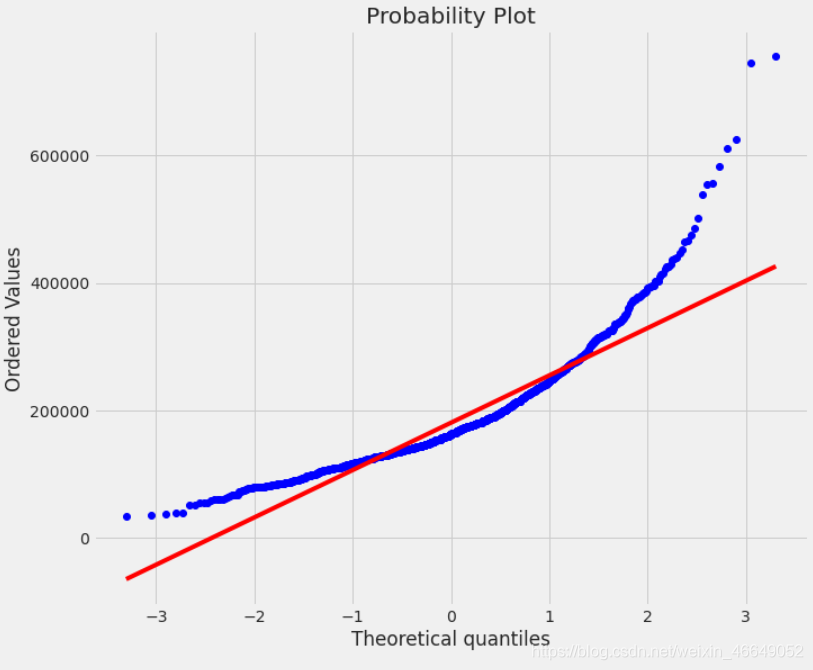
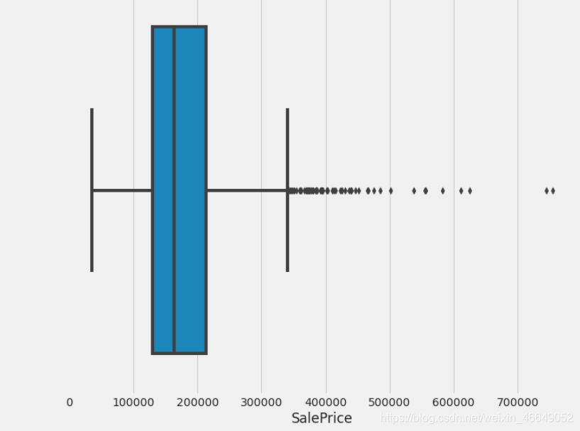
我们从上图可知,目标变量的分布不是正态分布;右偏(这里的左右指拖尾方向);
 最低0.47元/天 解锁文章


 684
684

 被折叠的 条评论
为什么被折叠?
被折叠的 条评论
为什么被折叠?
 到【灌水乐园】发言


